LINEPLOT
绘图 · 第 9 / 36 章
基础折线图
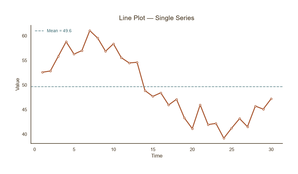
基础折线图
Python34 行
import matplotlib.pyplot as plt
import numpy as np

COLORS = ["#A8552E", "#35666E", "#D0A64F", "#3F2E18", "#7E8F52"]

np.random.seed(42)
x = np.arange(1, 31)
y = 50 + 8 * np.sin(x / 5) + np.random.normal(0, 2, len(x))

fig, ax = plt.subplots(figsize=(9, 5))

ax.plot(x, y, color=COLORS[0], linewidth=2.2,
        marker="o", markersize=4,
        markerfacecolor="white", markeredgecolor=COLORS[0],
        markeredgewidth=1.2, zorder=2)

# 均值参考线
ax.axhline(y.mean(), color=COLORS[1], linestyle="--",
           linewidth=1.5, alpha=0.7,
           label=f"Mean = {y.mean():.1f}")

ax.set_title("Line Plot — Single Series", fontsize=15, color=COLORS[3], pad=12)
ax.set_xlabel("Time", fontsize=12, color=COLORS[3])
ax.set_ylabel("Value", fontsize=12, color=COLORS[3])
ax.tick_params(axis="both", colors=COLORS[3])
ax.legend(frameon=False, fontsize=10, labelcolor=COLORS[1], loc="upper left")

for s in ("top", "right"):
    ax.spines[s].set_visible(False)
ax.spines["left"].set_color(COLORS[3])
ax.spines["bottom"].set_color(COLORS[3])

plt.tight_layout()
plt.show()多序列对比
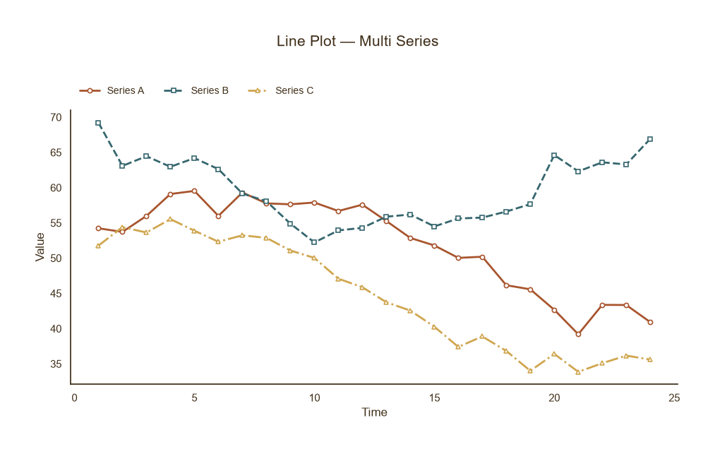
多序列对比
Python37 行
import matplotlib.pyplot as plt
import numpy as np

COLORS = ["#A8552E", "#35666E", "#D0A64F", "#3F2E18", "#7E8F52"]

np.random.seed(0)
x = np.arange(1, 25)
series = {
    "Series A": 50 + 8 * np.sin(x / 5) + np.random.normal(0, 1.5, len(x)),
    "Series B": 60 + 6 * np.cos(x / 4) + np.random.normal(0, 1.5, len(x)),
    "Series C": 45 + 10 * np.sin(x / 6 + 1) + np.random.normal(0, 1.5, len(x)),
}
linestyles = ["-", "--", "-."]
markers = ["o", "s", "^"]

fig, ax = plt.subplots(figsize=(9.5, 5.5))

for (name, y), c, ls, m in zip(series.items(), COLORS, linestyles, markers):
    ax.plot(x, y, color=c, linewidth=2.0,
            linestyle=ls, marker=m, markersize=4.5,
            markerfacecolor="white", markeredgecolor=c,
            markeredgewidth=1.2, label=name)

fig.suptitle("Line Plot — Multi Series", fontsize=15, color=COLORS[3], y=1.02)
ax.set_xlabel("Time", fontsize=12, color=COLORS[3])
ax.set_ylabel("Value", fontsize=12, color=COLORS[3])
ax.tick_params(axis="both", colors=COLORS[3])
ax.legend(frameon=False, fontsize=10, labelcolor=COLORS[3],
          loc="lower left", bbox_to_anchor=(0, 1.02),ncol=3)

for s in ("top", "right"):
    ax.spines[s].set_visible(False)
ax.spines["left"].set_color(COLORS[3])
ax.spines["bottom"].set_color(COLORS[3])

plt.tight_layout()
plt.show()带置信带 / 误差范围
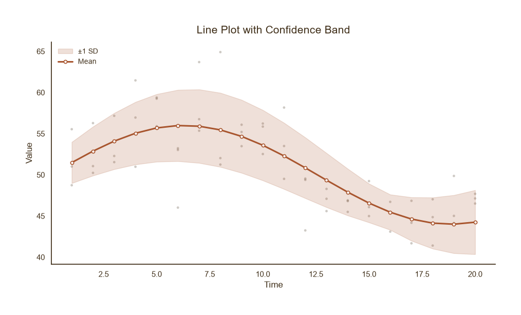
带置信带 / 误差范围
Python43 行
import matplotlib.pyplot as plt
import numpy as np

COLORS = ["#A8552E", "#35666E", "#D0A64F", "#3F2E18", "#7E8F52"]

np.random.seed(1)
x = np.arange(1, 21)
mean = 50 + 6 * np.sin(x / 4)
std = 2 + np.abs(np.sin(x / 5)) * 2.5

fig, ax = plt.subplots(figsize=(9.5, 5.5))

# 置信带(底层)
ax.fill_between(x, mean - std, mean + std,
                color=COLORS[0], alpha=0.18, zorder=1,
                label="±1 SD")

# 均值线(上层)
ax.plot(x, mean, color=COLORS[0], linewidth=2.2,
        marker="o", markersize=4.5,
        markerfacecolor="white", markeredgecolor=COLORS[0],
        markeredgewidth=1.2, zorder=2, label="Mean")

# 原始观测点(抽稀展示)
for _ in range(3):
    obs = mean + np.random.normal(0, std, len(x))
    ax.scatter(x, obs, s=12, color=COLORS[3],
               alpha=0.25, edgecolor="none", zorder=0)

ax.set_title("Line Plot with Confidence Band",
             fontsize=15, color=COLORS[3], pad=12)
ax.set_xlabel("Time", fontsize=12, color=COLORS[3])
ax.set_ylabel("Value", fontsize=12, color=COLORS[3])
ax.tick_params(axis="both", colors=COLORS[3])
ax.legend(frameon=False, fontsize=10, labelcolor=COLORS[3], loc="upper left")

for s in ("top", "right"):
    ax.spines[s].set_visible(False)
ax.spines["left"].set_color(COLORS[3])
ax.spines["bottom"].set_color(COLORS[3])

plt.tight_layout()
plt.show()双 Y 轴折线图
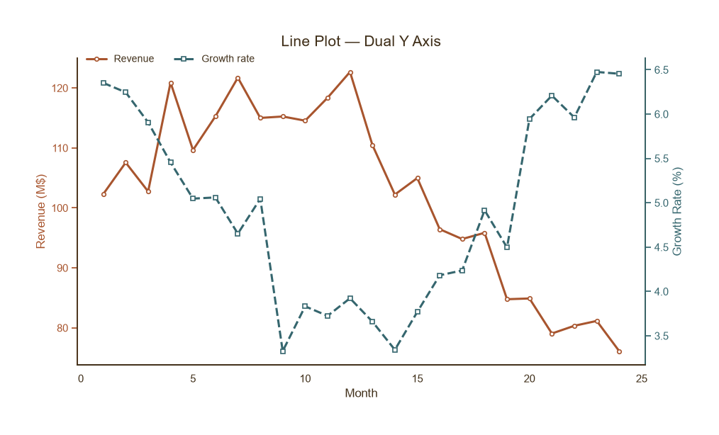
双 Y 轴折线图
Python47 行
import matplotlib.pyplot as plt
import numpy as np

COLORS = ["#A8552E", "#35666E", "#D0A64F", "#3F2E18", "#7E8F52"]

np.random.seed(2)
x = np.arange(1, 25)
revenue = 100 + 20 * np.sin(x / 5) + np.random.normal(0, 4, len(x))   # 百万
rate = 5 + 1.5 * np.cos(x / 4) + np.random.normal(0, 0.3, len(x))     # %

fig, ax1 = plt.subplots(figsize=(9.5, 5.5))

# 左轴
l1, = ax1.plot(x, revenue, color=COLORS[0], linewidth=2.2,
               marker="o", markersize=4, markerfacecolor="white",
               markeredgecolor=COLORS[0], markeredgewidth=1.2,
               label="Revenue")
ax1.set_xlabel("Month", fontsize=12, color=COLORS[3])
ax1.set_ylabel("Revenue (M$)", fontsize=12, color=COLORS[0])
ax1.tick_params(axis="y", colors=COLORS[0])
ax1.tick_params(axis="x", colors=COLORS[3])

# 右轴
ax2 = ax1.twinx()
l2, = ax2.plot(x, rate, color=COLORS[1], linewidth=2.2,
               linestyle="--", marker="s", markersize=4,
               markerfacecolor="white", markeredgecolor=COLORS[1],
               markeredgewidth=1.2, label="Growth rate")
ax2.set_ylabel("Growth Rate (%)", fontsize=12, color=COLORS[1])
ax2.tick_params(axis="y", colors=COLORS[1])

ax1.set_title("Line Plot — Dual Y Axis", fontsize=15, color=COLORS[3], pad=12)

# 合并图例
ax1.legend(handles=[l1, l2], frameon=False, fontsize=10,
           labelcolor=COLORS[3], loc="upper left",
           bbox_to_anchor=(0.0, 1.04), ncol=2)

for ax in (ax1, ax2):
    for s in ("top",):
        ax.spines[s].set_visible(False)
ax1.spines["left"].set_color(COLORS[0])
ax1.spines["bottom"].set_color(COLORS[3])
ax2.spines["right"].set_color(COLORS[1])

plt.tight_layout()
plt.show()分面折线图
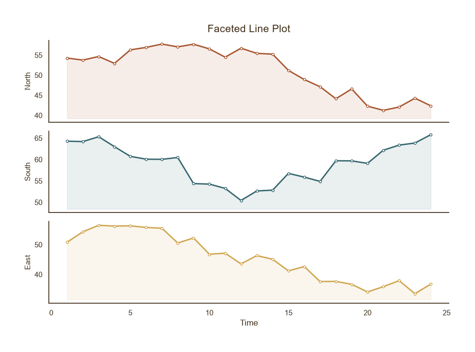
分面折线图
Python34 行
import matplotlib.pyplot as plt
import numpy as np

COLORS = ["#A8552E", "#35666E", "#D0A64F", "#3F2E18", "#7E8F52"]

np.random.seed(3)
x = np.arange(1, 25)
series = {
    "North": 50 + 8 * np.sin(x / 5) + np.random.normal(0, 1.5, len(x)),
    "South": 60 + 6 * np.cos(x / 4) + np.random.normal(0, 1.5, len(x)),
    "East":  45 + 10 * np.sin(x / 6 + 1) + np.random.normal(0, 1.5, len(x)),
}

fig, axes = plt.subplots(len(series), 1, figsize=(9, 6.5),
                         sharex=True)

for ax, (name, y), c in zip(axes, series.items(), COLORS):
    ax.plot(x, y, color=c, linewidth=2.0,
            marker="o", markersize=3.5,
            markerfacecolor="white", markeredgecolor=c,
            markeredgewidth=1.0)
    ax.fill_between(x, y, y.min() - 2, color=c, alpha=0.10)
    ax.set_ylabel(name, fontsize=11, color=COLORS[3])
    ax.tick_params(axis="both", colors=COLORS[3])
    for s in ("top", "right"):
        ax.spines[s].set_visible(False)
    ax.spines["left"].set_color(COLORS[3])
    ax.spines["bottom"].set_color(COLORS[3])

axes[-1].set_xlabel("Time", fontsize=12, color=COLORS[3])
axes[0].set_title("Faceted Line Plot", fontsize=15, color=COLORS[3], pad=12)

plt.tight_layout()
plt.show()