WORDCLOUD
绘图 · 第 22 / 36 章
基础词云(英文)
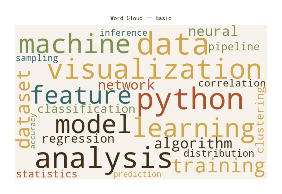
基础词云(英文)
Python42 行
import matplotlib.pyplot as plt
from wordcloud import WordCloud

COLORS = ["#A8552E", "#35666E", "#D0A64F", "#3F2E18", "#7E8F52"]
BG = "#F7F3EC"

# 词频字典
freq = {
    "data": 100, "python": 95, "analysis": 88, "visualization": 82,
    "machine": 75, "learning": 70, "model": 68, "feature": 62,
    "training": 58, "dataset": 55, "algorithm": 50, "neural": 48,
    "network": 46, "regression": 40, "classification": 38,
    "clustering": 35, "pipeline": 32, "statistics": 30,
    "correlation": 28, "distribution": 26, "sampling": 22,
    "inference": 20, "prediction": 18, "accuracy": 16,
}

# 颜色函数:从主题色中循环取值
def theme_color_func(word, font_size, position, orientation, random_state=None, **kwargs):
    return COLORS[hash(word) % len(COLORS)]

wc = WordCloud(
    width=900, height=550,
    background_color=BG,
    color_func=theme_color_func,
    max_words=100,
    prefer_horizontal=0.85,     # 85% 的词水平排列
    relative_scaling=0.5,       # 字号与频率的关联度
    min_font_size=10,
    max_font_size=110,
    random_state=42,
).generate_from_frequencies(freq)

fig, ax = plt.subplots(figsize=(10, 6))

ax.imshow(wc, interpolation="bilinear")
ax.axis("off")

ax.set_title("Word Cloud — Basic", fontsize=16, color=COLORS[3], pad=12)

plt.tight_layout()
plt.show()中文词云
中文词云
Python53 行
import matplotlib.pyplot as plt
from wordcloud import WordCloud
import jieba
from collections import Counter

COLORS = ["#A8552E", "#35666E", "#D0A64F", "#3F2E18", "#7E8F52"]
BG = "#F7F3EC"

# 中文文本
text = """
数据可视化 是 数据分析 的 重要 环节 通过 图表 展示 数据 规律
Python 是 数据科学 的 主流 工具 支持 数据清洗 统计分析 机器学习
可视化 图表 包括 折线图 柱状图 散点图 热力图 词云 等多种 形式
好的 可视化 应该 清晰 准确 美观 帮助 读者 快速 理解 数据
数据 分析 流程 包括 数据采集 数据清洗 特征工程 建模 评估
机器学习 模型 需要 训练 验证 测试 避免 过拟合 欠拟合
"""

# 分词 + 词频统计
words = jieba.lcut(text)
words = [w.strip() for w in words if len(w.strip()) > 1]
freq = Counter(words)

# 颜色函数
def theme_color_func(word, font_size, position, orientation, random_state=None, **kwargs):
    return COLORS[hash(word) % len(COLORS)]

wc = WordCloud(
    width=900, height=550,
    background_color=BG,
    font_path="/System/Library/Fonts/PingFang.ttc",   # macOS 中文字体
    # font_path="C:/Windows/Fonts/msyh.ttc",          # Windows 微软雅黑
    # font_path="/usr/share/fonts/truetype/wqy/wqy-microhei.ttc",  # Linux 文泉驿
    color_func=theme_color_func,
    max_words=80,
    prefer_horizontal=0.9,
    relative_scaling=0.5,
    min_font_size=12,
    max_font_size=120,
    random_state=42,
).generate_from_frequencies(freq)

fig, ax = plt.subplots(figsize=(10, 6))

ax.imshow(wc, interpolation="bilinear")
ax.axis("off")

ax.set_title("中文词云 — Chinese Word Cloud",
             fontsize=16, color=COLORS[3], pad=12,
             fontproperties=None)   # 若标题要中文,需指定字体

plt.tight_layout()
plt.show()带遮罩形状的词云
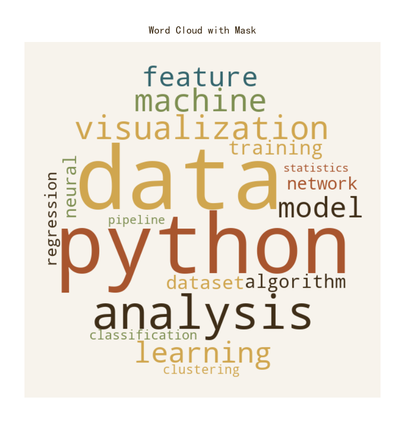
带遮罩形状的词云
Python44 行
import matplotlib.pyplot as plt
from wordcloud import WordCloud
import numpy as np
from PIL import Image

COLORS = ["#A8552E", "#35666E", "#D0A64F", "#3F2E18", "#7E8F52"]
BG = "#F7F3EC"

# 构造一个简单的圆形遮罩(实际使用可加载 PNG 图)
x, y = np.ogrid[:600, :600]
mask = ((x - 300) ** 2 + (y - 300) ** 2 > 280 ** 2) * 255
mask = mask.astype(np.uint8)

freq = {
    "data": 100, "python": 95, "analysis": 88, "visualization": 82,
    "machine": 75, "learning": 70, "model": 68, "feature": 62,
    "training": 58, "dataset": 55, "algorithm": 50, "neural": 48,
    "network": 46, "regression": 40, "classification": 38,
    "clustering": 35, "pipeline": 32, "statistics": 30,
}

def theme_color_func(word, font_size, position, orientation, random_state=None, **kwargs):
    return COLORS[hash(word) % len(COLORS)]

wc = WordCloud(
    width=600, height=600,
    background_color=BG,
    mask=mask,
    color_func=theme_color_func,
    max_words=100,
    prefer_horizontal=0.85,
    relative_scaling=0.5,
    random_state=42,
).generate_from_frequencies(freq)

fig, ax = plt.subplots(figsize=(8, 8))

ax.imshow(wc, interpolation="bilinear")
ax.axis("off")

ax.set_title("Word Cloud with Mask", fontsize=16, color=COLORS[3], pad=12)

plt.tight_layout()
plt.show()单色渐变词云
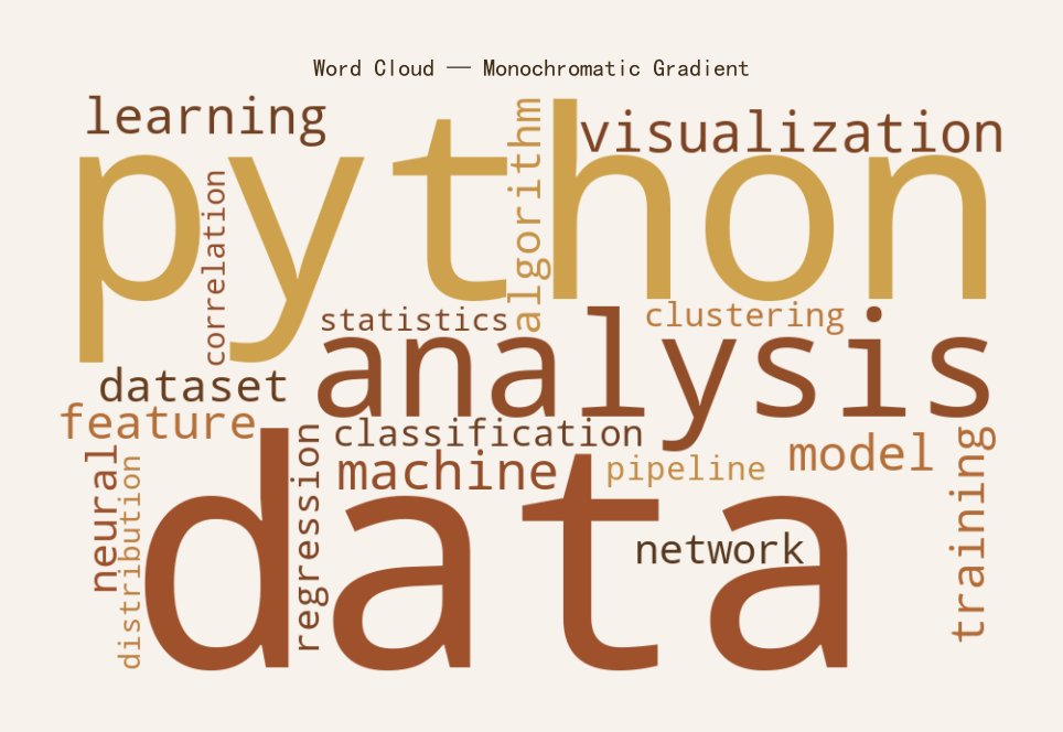
单色渐变词云
Python41 行
import matplotlib.pyplot as plt
from wordcloud import WordCloud
import numpy as np
from matplotlib.colors import LinearSegmentedColormap

BG = "#F7F3EC"
CMAP = LinearSegmentedColormap.from_list(
    "theme", ["#D0A64F", "#A8552E", "#3F2E18"], N=256
)

freq = {
    "data": 100, "python": 95, "analysis": 88, "visualization": 82,
    "machine": 75, "learning": 70, "model": 68, "feature": 62,
    "training": 58, "dataset": 55, "algorithm": 50, "neural": 48,
    "network": 46, "regression": 40, "classification": 38,
    "clustering": 35, "pipeline": 32, "statistics": 30,
    "correlation": 28, "distribution": 26,
}

wc = WordCloud(
    width=900, height=550,
    background_color=BG,
    colormap=CMAP,               # 用渐变替代离散色
    max_words=100,
    prefer_horizontal=0.85,
    relative_scaling=0.5,
    random_state=42,
).generate_from_frequencies(freq)

fig, ax = plt.subplots(figsize=(10, 6))
fig.patch.set_facecolor(BG)
ax.set_facecolor(BG)

ax.imshow(wc, interpolation="bilinear")
ax.axis("off")

ax.set_title("Word Cloud — Monochromatic Gradient",
             fontsize=16, color="#3F2E18", pad=12)

plt.tight_layout()
plt.show()词云 + 词频条形图
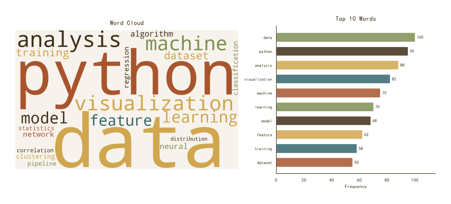
词云 + 词频条形图
Python72 行
import matplotlib.pyplot as plt
from wordcloud import WordCloud
from matplotlib.gridspec import GridSpec

COLORS = ["#A8552E", "#35666E", "#D0A64F", "#3F2E18", "#7E8F52"]
BG = "#F7F3EC"

freq = {
    "data": 100, "python": 95, "analysis": 88, "visualization": 82,
    "machine": 75, "learning": 70, "model": 68, "feature": 62,
    "training": 58, "dataset": 55, "algorithm": 50, "neural": 48,
    "network": 46, "regression": 40, "classification": 38,
    "clustering": 35, "pipeline": 32, "statistics": 30,
    "correlation": 28, "distribution": 26,
}

def theme_color_func(word, font_size, position, orientation, random_state=None, **kwargs):
    return COLORS[hash(word) % len(COLORS)]

wc = WordCloud(
    width=800, height=500,
    background_color=BG,
    color_func=theme_color_func,
    max_words=100,
    prefer_horizontal=0.85,
    random_state=42,
).generate_from_frequencies(freq)

# 取 Top 10
top10 = sorted(freq.items(), key=lambda x: x[1], reverse=True)[:10]
words_top = [w for w, _ in top10][::-1]
vals_top = [v for _, v in top10][::-1]

fig = plt.figure(figsize=(14, 6))
gs = GridSpec(1, 2, width_ratios=[1.4, 1], figure=fig)

# 左:词云
ax1 = fig.add_subplot(gs[0, 0])
ax1.imshow(wc, interpolation="bilinear")
ax1.axis("off")
ax1.set_title("Word Cloud", fontsize=15, color=COLORS[3], pad=12)

# 右:Top 10 条形图
ax2 = fig.add_subplot(gs[0, 1])

y_pos = range(len(words_top))
bars = ax2.barh(y_pos, vals_top,
                color=[COLORS[i % len(COLORS)] for i in range(len(words_top))],
                alpha=0.85, edgecolor="white", linewidth=1.0,
                height=0.65)

for bar, v in zip(bars, vals_top):
    ax2.text(bar.get_width() + 1.5,
             bar.get_y() + bar.get_height() / 2,
             f"{v}", va="center", ha="left",
             fontsize=10, color=COLORS[3])

ax2.set_yticks(y_pos)
ax2.set_yticklabels(words_top, fontsize=10)
ax2.set_xlim(0, max(vals_top) * 1.15)

ax2.set_title("Top 10 Words", fontsize=15, color=COLORS[3], pad=12)
ax2.set_xlabel("Frequency", fontsize=11, color=COLORS[3])
ax2.tick_params(axis="both", colors=COLORS[3])

for s in ("top", "right"):
    ax2.spines[s].set_visible(False)
ax2.spines["left"].set_color(COLORS[3])
ax2.spines["bottom"].set_color(COLORS[3])

plt.tight_layout()
plt.show()