直方图

直方图（一维分布）hist()

hist() 干三件事：分箱 → 计数 → 画柱子。它同时是一个统计工具和一个绘图工具，所以参数分两类：一类决定「怎么分箱」（bins range weights），一类决定「怎么画」（histtype density cumulative rwidth）。

Axes.hist(
    x,                    # 数据：一维数组，或多个数组组成的列表（一次画多组）
    bins=None,            # 箱数(int) / 边界数组 / "auto" 等字符串；None → rcParams["hist.bins"]=10
    range=None,           # (min, max) 统计范围，范围外的数据直接丢掉
    density=False,        # True 时纵轴是概率密度，总面积 = 1
    weights=None,         # 与 x 等长的权重数组，做加权计数
    cumulative=False,     # True 从左往右累加；-1 从右往左
    bottom=None,          # 柱子的起始高度，堆叠用
    histtype='bar',       # bar / barstacked / step / stepfilled
    align='mid',          # 箱边界与刻度对齐方式：mid / left / right
    orientation='vertical',  # vertical / horizontal
    rwidth=None,          # 柱宽占箱宽的比例，<1 会留缝
    log=False,            # 纵轴取对数
    color=None,           # 填充色
    label=None,           # 图例文字
    stacked=False,        # 多组数据时是否堆叠
    data=None,            # 允许 x 传列名（配 pandas）
    **kwargs              # 其余键传给每根柱子（Patch）
)

最小示例

import numpy as np
import matplotlib.pyplot as plt

rng = np.random.default_rng(42)
data = rng.normal(0, 1, 2000)          # 2000 个标准正态样本
data_b = rng.normal(2, 1.2, 1200)      # 第二组，后面几节要用

fig, ax = plt.subplots()
ax.hist(data, bins=30)
plt.show()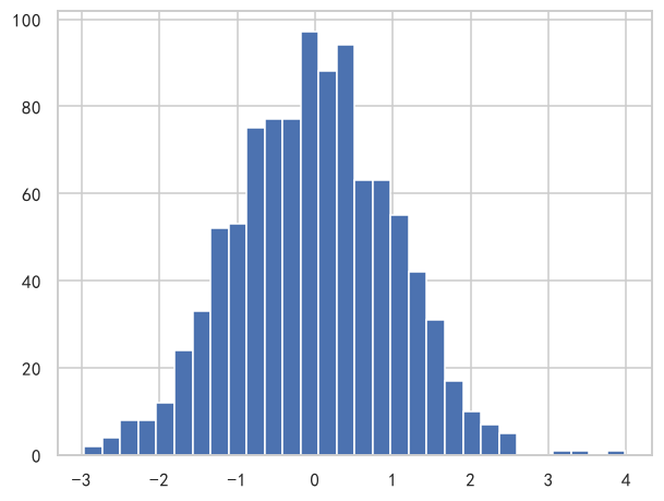

bins：形状由它决定

ax.hist(data, bins=5)                          # 太粗，双峰会被抹平成单峰
ax.hist(data, bins=10)                         # 默认值（rcParams["hist.bins"]）
ax.hist(data, bins=30)                         # 常用
ax.hist(data, bins="auto")                     # 按数据量自动挑，最省事
ax.hist(data, bins=[-3, -1, 0, 1, 3])          # 自己给边界（可不等宽）
ax.hist(data, bins=np.arange(-4, 4.5, 0.5))    # 等宽边界的写法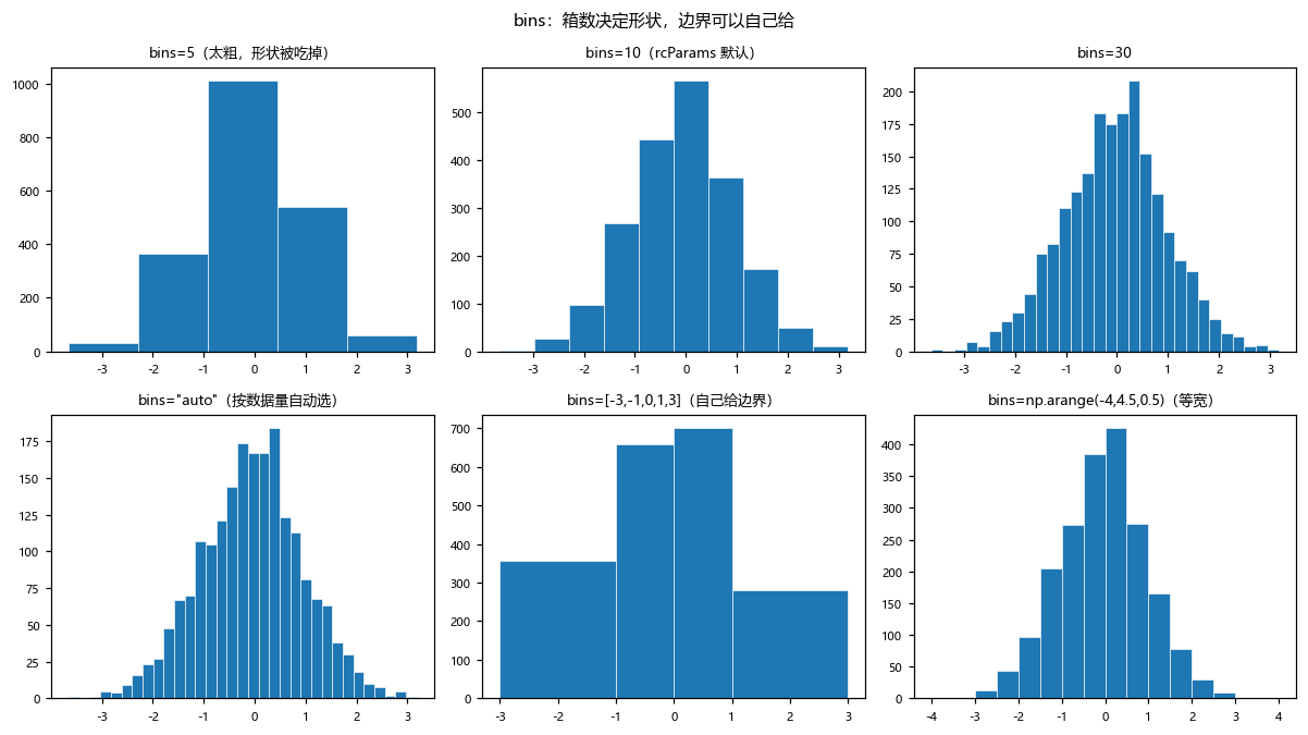

三种给法各自的适用场景：

跨图对比时必须固定边界。 两张图各自 bins=30，箱子边界并不一样，柱子高度无法直接比。要对比就共用一个 edges：

edges = np.linspace(-4, 4, 33)
ax.hist(data, bins=edges, alpha=0.6)
ax.hist(data_b, bins=edges, alpha=0.6)

range：先砍数据，再分箱

ax.hist(data, bins=30, range=(-2, 2))

range 之外的数据直接丢弃，不参与计数，也不会在图上留空箱。所以它既是「剔除极值影响」的手段，也是「两图共用同一坐标系」的技巧——配合同一组 bins 使用。

注意 range 与 bins 的边界会互相影响：给了 bins=[-3,-1,0,1,3] 又给 range=(-2,2)，实际生效的是 bins 的边界。

density：纵轴换成密度

ax.hist(data, bins=30)                      # 纵轴：计数（最高 200 左右）
ax.hist(data, bins=30, density=True)        # 纵轴：密度（总面积 = 1）

xs = np.linspace(-4, 4, 200)
ax.plot(xs, np.exp(-xs ** 2 / 2) / np.sqrt(2 * np.pi), "r-", lw=1.5)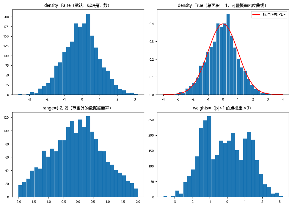

只有开了 density=True，直方图才能和概率密度曲线画在同一张图上——否则一个是「个数」一个是「密度」，量纲不同，曲线会被压成贴着 x 轴的一条线。

density=True 的效果是 sum(n * 箱宽) == 1，不是 sum(n) == 1。箱宽不同时，高箱不一定计数多。

weights：加权计数

w = np.where(np.abs(data) > 1, 3.0, 1.0)    # |x|>1 的点算 3 个
ax.hist(data, bins=30, weights=w)

weights 与 x 等长，默认全 1。常见用法：抽样权重、金额加权（每个点的「高度」是金额而不是笔数）。注意 density=True 时权重也会被归一进来，两者可以同用。

cumulative：累积分布

ax.hist(data, bins=30, cumulative=True)     # 从左往右累加，右端 = 总数
ax.hist(data, bins=30, cumulative=-1)       # 从右往左累，左端 = 总数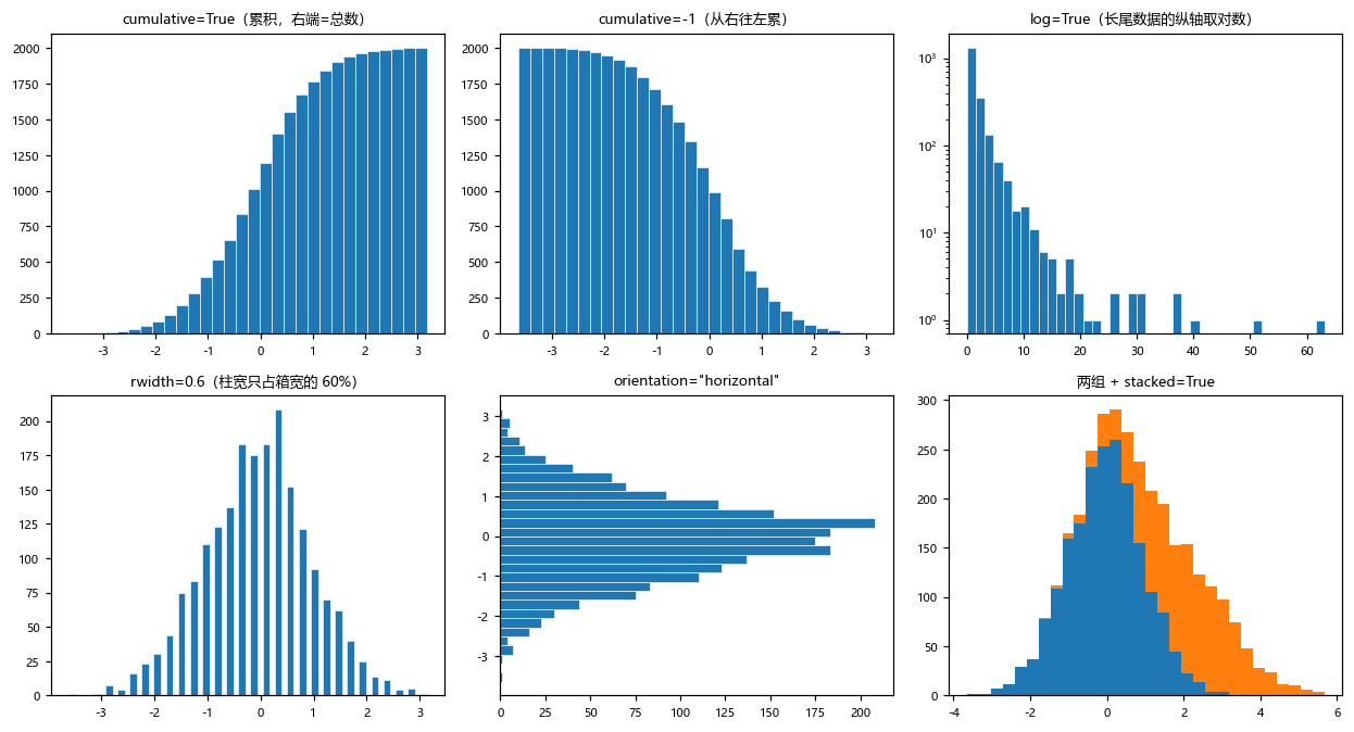

cumulative=True 的柱高是「小于等于当前箱右边界的数据个数」。想看中位数在哪，找柱高 = 总数一半的位置即可；cumulative=-1 则是「大于多少」，看尾部更直观。

想要真正平滑的累积曲线，ax.ecdf(data) 比 hist(cumulative=True) 更合适 —— 它直接画累积分布（complementary=True 就是反向累积，等价于 hist(cumulative=-1)），不用自己算箱。

histtype：四种柱形

ax.hist(data, bins=30, histtype="bar")            # 默认：实心柱
ax.hist([data, data_b], bins=30, histtype="barstacked")   # 堆叠柱
ax.hist(data, bins=30, histtype="step")           # 只有阶梯轮廓线
ax.hist(data, bins=30, histtype="stepfilled")     # 阶梯 + 填充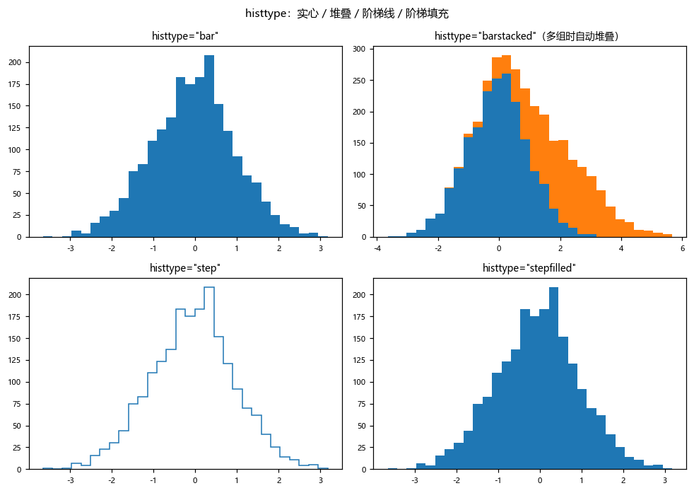

实际选择：

• 多组数据叠在一张图上，用 "step"。实心柱会互相遮挡，阶梯线才能看出各自形状。
• 要显示构成比例，用 "barstacked" 配多组数据（等价于 stacked=True + histtype="bar"）。
• "stepfilled" 适合单组数据，比 "bar" 干净。

orientation / rwidth / log

ax.hist(data, bins=30, orientation="horizontal")   # 横向直方图，x 轴变计数
ax.hist(data, bins=30, rwidth=0.6)                 # 柱宽只占箱宽 60%，柱间留缝
ax.hist(long_tail_data, bins=40, log=True)         # 长尾数据：纵轴取对数

log=True 值得单独记：长尾数据（如金额、访问量）用线性纵轴时，除了最高那根柱，其余全被压成一条线。取对数后尾部才看得见——但代价是「柱高的视觉比例」不再是真实比例，读图时要留心。

stacked 与 align

ax.hist([data, data_b], bins=30, stacked=True)     # 两组堆叠，总高度是两组之和

ax.hist(data, bins=30, align="mid")                # 默认：刻度在箱子中心
ax.hist(data, bins=30, align="left")               # 刻度在箱子左边界
ax.hist(data, bins=30, align="right")              # 刻度在箱子右边界

align 在单张图上看不出差别，但叠加密度曲线或竖线时会错半格。默认 "mid" 表示刻度落在箱子中心（即 (边界[i] + 边界[i+1]) / 2），而箱边界本身在 边界[i] 上。要在箱边界画竖线，就得用 align="left" 或者手动按边界算坐标。

返回的三元组

hist() 返回 (n, bins, patches)：

n, bins, patches = ax.hist(data, bins=30)
# n       : 每箱计数，dtype 恒为 float（即使没做归一化）
# bins    : 箱边界，长度 = 箱数 + 1
# patches : BarContainer，可迭代取每根柱子改样式

print(n.sum())                  # == len(data)（没设 range/weights 时）
print(np.diff(bins))            # 各箱宽度
for patch, count in zip(patches, n):
    patch.set_alpha(count / n.max())     # 按计数调透明度

拿到 n 和 bins 就能做二次加工：找众数所在箱、标注峰顶、把计数写回图里。

注意事项

• bins 默认只有 10。 数据量上千时必须显式给，否则形状不可信。
• n 的 dtype 是 float，n.sum() 与 len(data) 相等但不一定是整数类型。
• 跨图对比要共用 edges。 各自 bins=30 的箱边界互不相同。
• density=True 满足的是 sum(n * width) == 1，不是 sum(n) == 1。
• range 之外的数据被丢弃，不报错。
• 多组数据用 histtype="step"，否则实心柱互相遮挡。
• align 影响刻度与箱边界的对齐，叠加竖线时要留意半格偏移。