SPIDERPLOT
绘图 · 第 30 / 36 章
基础雷达图
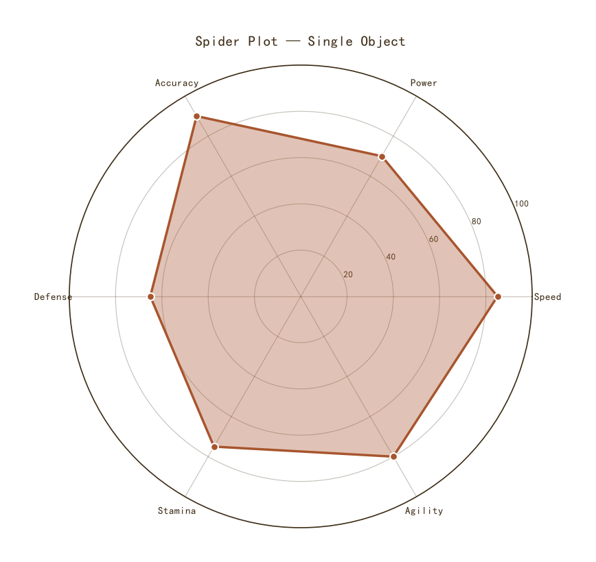
基础雷达图
Python50 行
import matplotlib.pyplot as plt
import numpy as np

COLORS = ["#A8552E", "#35666E", "#D0A64F", "#3F2E18", "#7E8F52"]
BG = "#F7F3EC"

# 6 个维度
categories = ["Speed", "Power", "Accuracy", "Defense", "Stamina", "Agility"]
values = [85, 70, 90, 65, 75, 80]

# 闭合:首尾相连
values_closed = values + [values[0]]

# 计算角度
n = len(categories)
angles = np.linspace(0, 2 * np.pi, n, endpoint=False).tolist()
angles_closed = angles + [angles[0]]

fig, ax = plt.subplots(figsize=(8, 8), subplot_kw={"projection": "polar"})

# 画线 + 填充
ax.plot(angles_closed, values_closed,
        color=COLORS[0], linewidth=2.5)
ax.fill(angles_closed, values_closed,
        color=COLORS[0], alpha=0.35)

# 顶点标记
ax.scatter(angles, values, s=60, color=COLORS[0],
           edgecolor="white", linewidth=1.5, zorder=5)

# 角度标签
ax.set_xticks(angles)
ax.set_xticklabels(categories, fontsize=11, color=COLORS[3])

# 半径范围
ax.set_ylim(0, 100)
ax.set_yticks([20, 40, 60, 80, 100])
ax.set_yticklabels(["20", "40", "60", "80", "100"],
                   fontsize=9, color=COLORS[3])

# 网格样式
ax.grid(color=COLORS[3], linewidth=0.8, alpha=0.3)
ax.spines["polar"].set_color(COLORS[3])
ax.spines["polar"].set_linewidth(1.2)

ax.set_title("Spider Plot — Single Object",
             fontsize=15, color=COLORS[3], pad=20)

plt.tight_layout()
plt.show()多对象对比
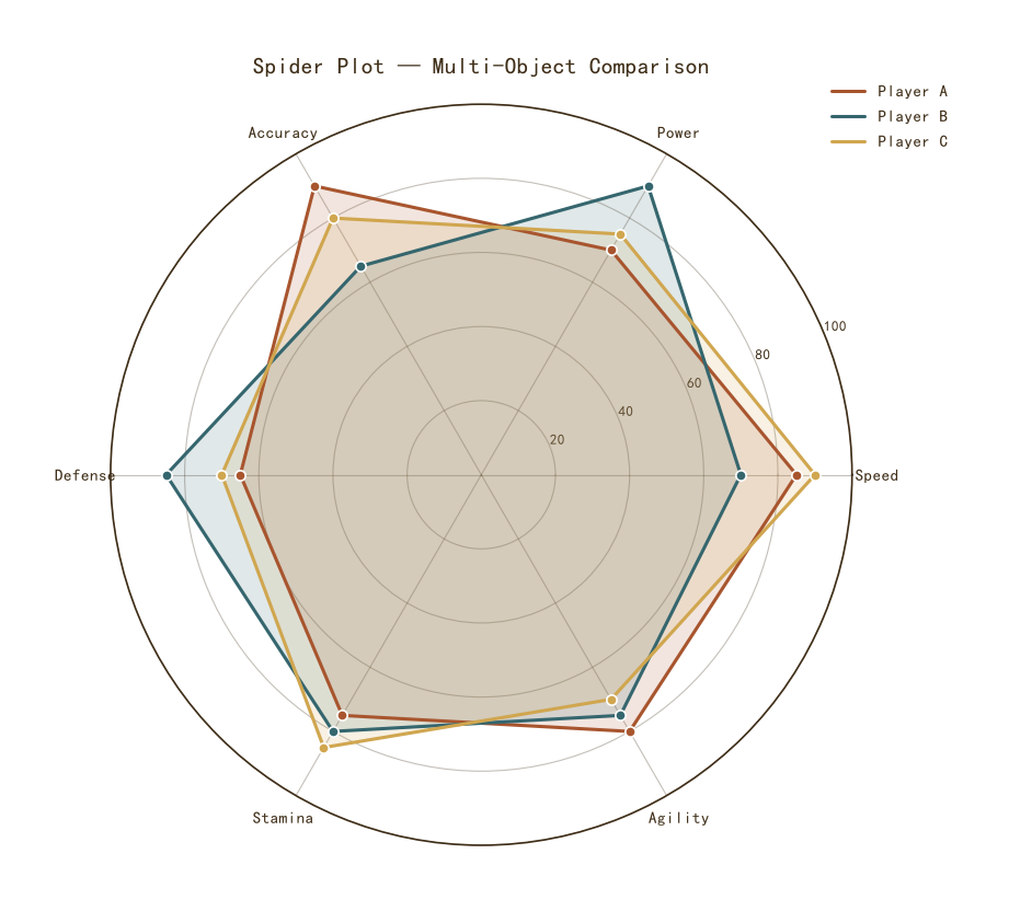
多对象对比
Python47 行
import matplotlib.pyplot as plt
import numpy as np

COLORS = ["#A8552E", "#35666E", "#D0A64F", "#3F2E18", "#7E8F52"]
BG = "#F7F3EC"

categories = ["Speed", "Power", "Accuracy", "Defense", "Stamina", "Agility"]

data = {
    "Player A": [85, 70, 90, 65, 75, 80],
    "Player B": [70, 90, 65, 85, 80, 75],
    "Player C": [90, 75, 80, 70, 85, 70],
}

n = len(categories)
angles = np.linspace(0, 2 * np.pi, n, endpoint=False).tolist()
angles_closed = angles + [angles[0]]

fig, ax = plt.subplots(figsize=(8.5, 8.5), subplot_kw={"projection": "polar"})

for (name, vals), c in zip(data.items(), COLORS):
    vals_closed = vals + [vals[0]]
    ax.plot(angles_closed, vals_closed,
            color=c, linewidth=2.2, label=name)
    ax.fill(angles_closed, vals_closed, color=c, alpha=0.15)
    ax.scatter(angles, vals, s=45, color=c,
               edgecolor="white", linewidth=1.2, zorder=5)

ax.set_xticks(angles)
ax.set_xticklabels(categories, fontsize=11, color=COLORS[3])

ax.set_ylim(0, 100)
ax.set_yticks([20, 40, 60, 80, 100])
ax.set_yticklabels(["20", "40", "60", "80", "100"],
                   fontsize=9, color=COLORS[3])

ax.grid(color=COLORS[3], linewidth=0.8, alpha=0.3)
ax.spines["polar"].set_color(COLORS[3])
ax.spines["polar"].set_linewidth(1.2)

ax.set_title("Spider Plot — Multi-Object Comparison",
             fontsize=15, color=COLORS[3], pad=20)
ax.legend(frameon=False, fontsize=11, labelcolor=COLORS[3],
          loc="upper right", bbox_to_anchor=(1.15, 1.05))

plt.tight_layout()
plt.show()带基准线的雷达图
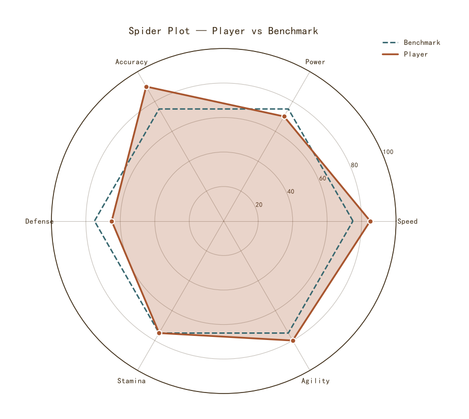
带基准线的雷达图
Python49 行
import matplotlib.pyplot as plt
import numpy as np

COLORS = ["#A8552E", "#35666E", "#D0A64F", "#3F2E18", "#7E8F52"]
BG = "#F7F3EC"

categories = ["Speed", "Power", "Accuracy", "Defense", "Stamina", "Agility"]
player = [85, 70, 90, 65, 75, 80]
benchmark = [75, 75, 75, 75, 75, 75]

n = len(categories)
angles = np.linspace(0, 2 * np.pi, n, endpoint=False).tolist()
angles_closed = angles + [angles[0]]

fig, ax = plt.subplots(figsize=(8.5, 8.5), subplot_kw={"projection": "polar"})

# 基准线(虚线)
ax.plot(angles_closed, benchmark + [benchmark[0]],
        color=COLORS[1], linewidth=2.0,
        linestyle="--", label="Benchmark")

# 玩家数据
player_closed = player + [player[0]]
ax.plot(angles_closed, player_closed,
        color=COLORS[0], linewidth=2.5, label="Player")
ax.fill(angles_closed, player_closed,
        color=COLORS[0], alpha=0.25)
ax.scatter(angles, player, s=55, color=COLORS[0],
           edgecolor="white", linewidth=1.5, zorder=5)

ax.set_xticks(angles)
ax.set_xticklabels(categories, fontsize=11, color=COLORS[3])

ax.set_ylim(0, 100)
ax.set_yticks([20, 40, 60, 80, 100])
ax.set_yticklabels(["20", "40", "60", "80", "100"],
                   fontsize=9, color=COLORS[3])

ax.grid(color=COLORS[3], linewidth=0.8, alpha=0.3)
ax.spines["polar"].set_color(COLORS[3])
ax.spines["polar"].set_linewidth(1.2)

ax.set_title("Spider Plot — Player vs Benchmark",
             fontsize=15, color=COLORS[3], pad=20)
ax.legend(frameon=False, fontsize=11, labelcolor=COLORS[3],
          loc="upper right", bbox_to_anchor=(1.15, 1.05))

plt.tight_layout()
plt.show()