DENSITY PLOT
绘图 · 第 2 / 36 章
单组密度图
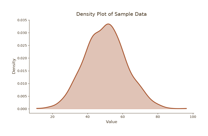
单组密度图
Python33 行
import matplotlib.pyplot as plt
import numpy as np

COLORS = ["#A8552E", "#35666E", "#D0A64F", "#3F2E18", "#7E8F52"]
BG = "#F7F3EC"

np.random.seed(42)
data = np.random.normal(loc=50, scale=12, size=1000)

fig, ax = plt.subplots(figsize=(8, 5))
# fig.patch.set_facecolor(BG)
# ax.set_facecolor(BG)

# 核密度估计(手写高斯核,避免依赖 scipy)
from scipy.stats import gaussian_kde
kde = gaussian_kde(data)
xs = np.linspace(data.min(), data.max(), 300)

ax.fill_between(xs, kde(xs), color=COLORS[0], alpha=0.35)
ax.plot(xs, kde(xs), color=COLORS[0], linewidth=2.5, label="Density")

ax.set_title("Density Plot of Sample Data", fontsize=15, color=COLORS[3], pad=12)
ax.set_xlabel("Value", fontsize=12, color=COLORS[3])
ax.set_ylabel("Density", fontsize=12, color=COLORS[3])
ax.tick_params(axis="both", colors=COLORS[3])

for s in ("top", "right"):
    ax.spines[s].set_visible(False)
ax.spines["left"].set_color(COLORS[3])
ax.spines["bottom"].set_color(COLORS[3])

plt.tight_layout()
plt.show()多组密度对比
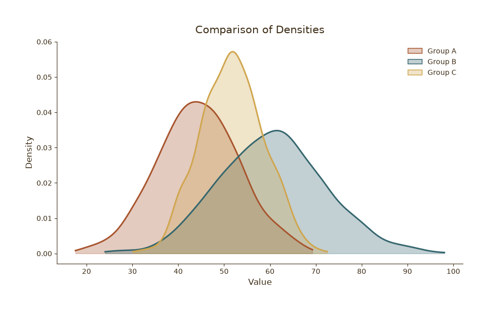
多组密度对比
Python50 行
import matplotlib.pyplot as plt
import numpy as np
from matplotlib.patches import Patch
from matplotlib.colors import to_rgba
from scipy.stats import gaussian_kde

COLORS = ["#A8552E", "#35666E", "#D0A64F", "#3F2E18", "#7E8F52"]

np.random.seed(0)
groups = {
    "Group A": np.random.normal(45, 9, 800),
    "Group B": np.random.normal(60, 12, 800),
    "Group C": np.random.normal(52, 7, 800),
}

fig, ax = plt.subplots(figsize=(9, 5.5))

fill_alpha = 0.30   # 内部:高透明
edge_alpha = 0.9    # 边框:几乎不透明

for (name, values), c in zip(groups.items(), COLORS):
    kde = gaussian_kde(values)
    xs = np.linspace(values.min(), values.max(), 300)
    ax.fill_between(xs, kde(xs), color=c, alpha=fill_alpha)
    ax.plot(xs, kde(xs), color=c, linewidth=2.2)

# 手动构造图例句柄:填充高透明,边框低透明
handles = [
    Patch(
        facecolor=to_rgba(c, fill_alpha),   # 内部:透明
        edgecolor=to_rgba(c, edge_alpha),   # 边框:不透明
        linewidth=1.2,
        label=name,
    )
    for name, c in zip(groups.keys(), COLORS)
]

ax.set_title("Comparison of Densities", fontsize=15, color=COLORS[3], pad=12)
ax.set_xlabel("Value", fontsize=12, color=COLORS[3])
ax.set_ylabel("Density", fontsize=12, color=COLORS[3])
ax.tick_params(axis="both", colors=COLORS[3])
ax.legend(handles=handles, frameon=False, fontsize=10, labelcolor=COLORS[3])

for s in ("top", "right"):
    ax.spines[s].set_visible(False)
ax.spines["left"].set_color(COLORS[3])
ax.spines["bottom"].set_color(COLORS[3])

plt.tight_layout()
plt.show()密度图 + 直方图叠加
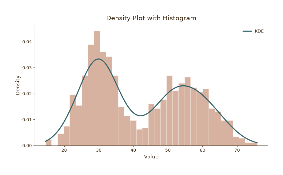
密度图 + 直方图叠加
Python40 行
import matplotlib.pyplot as plt
import numpy as np
from scipy.stats import gaussian_kde

COLORS = ["#A8552E", "#35666E", "#D0A64F", "#3F2E18", "#7E8F52"]
BG = "#F7F3EC"

np.random.seed(7)
data = np.concatenate([
    np.random.normal(30, 5, 500),
    np.random.normal(55, 8, 500),
])

fig, ax = plt.subplots(figsize=(8.5, 5))
# fig.patch.set_facecolor(BG)
# ax.set_facecolor(BG)

# 直方图(归一化为密度)
ax.hist(data, bins=35, density=True,
        color=COLORS[0], alpha=0.45,
        edgecolor="white", linewidth=0.6)

# 密度曲线
kde = gaussian_kde(data)
xs = np.linspace(data.min(), data.max(), 400)
ax.plot(xs, kde(xs), color=COLORS[1], linewidth=2.5, label="KDE")

ax.set_title("Density Plot with Histogram", fontsize=15, color=COLORS[3], pad=12)
ax.set_xlabel("Value", fontsize=12, color=COLORS[3])
ax.set_ylabel("Density", fontsize=12, color=COLORS[3])
ax.tick_params(axis="both", colors=COLORS[3])
ax.legend(frameon=False, fontsize=10, labelcolor=COLORS[3])

for s in ("top", "right"):
    ax.spines[s].set_visible(False)
ax.spines["left"].set_color(COLORS[3])
ax.spines["bottom"].set_color(COLORS[3])

plt.tight_layout()
plt.show()