SCATTER PLOT
绘图 · 第 4 / 36 章
单组散点图
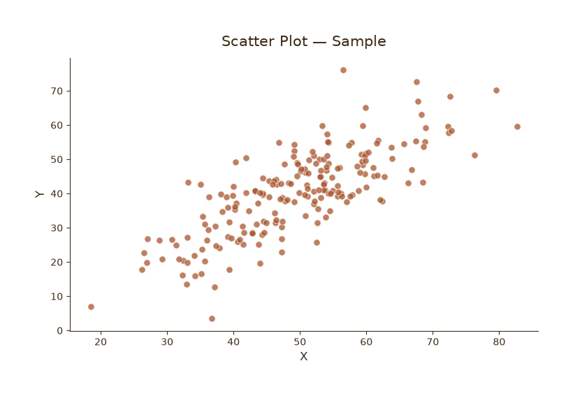
单组散点图
Python27 行
import matplotlib.pyplot as plt
import numpy as np

COLORS = ["#A8552E", "#35666E", "#D0A64F", "#3F2E18", "#7E8F52"]

np.random.seed(42)
n = 200
x = np.random.normal(50, 12, n)
y = 0.8 * x + np.random.normal(0, 8, n)

fig, ax = plt.subplots(figsize=(7.5, 5))

ax.scatter(x, y, s=45, color=COLORS[0],
           edgecolor="white", linewidth=0.6, alpha=0.75)

ax.set_title("Scatter Plot — Sample", fontsize=15, color=COLORS[3], pad=12)
ax.set_xlabel("X", fontsize=12, color=COLORS[3])
ax.set_ylabel("Y", fontsize=12, color=COLORS[3])
ax.tick_params(axis="both", colors=COLORS[3])

for s in ("top", "right"):
    ax.spines[s].set_visible(False)
ax.spines["left"].set_color(COLORS[3])
ax.spines["bottom"].set_color(COLORS[3])

plt.tight_layout()
plt.show()按分类着色
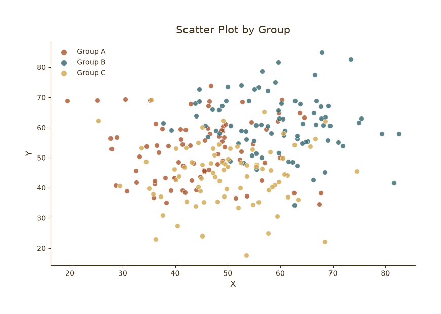
按分类着色
Python32 行
import matplotlib.pyplot as plt
import numpy as np

COLORS = ["#A8552E", "#35666E", "#D0A64F", "#3F2E18", "#7E8F52"]

np.random.seed(0)
groups = {
    "Group A": (np.random.normal(45, 10, 80), np.random.normal(50, 10, 80)),
    "Group B": (np.random.normal(60, 10, 80), np.random.normal(62, 10, 80)),
    "Group C": (np.random.normal(52, 10, 80), np.random.normal(45, 10, 80)),
}

fig, ax = plt.subplots(figsize=(8, 5.5))

for (name, (x, y)), c in zip(groups.items(), COLORS):
    ax.scatter(x, y, s=50, color=c, edgecolor="white",
               linewidth=0.6, alpha=0.8, label=name)

ax.set_title("Scatter Plot by Group", fontsize=15, color=COLORS[3], pad=12)
ax.set_xlabel("X", fontsize=12, color=COLORS[3])
ax.set_ylabel("Y", fontsize=12, color=COLORS[3])
ax.tick_params(axis="both", colors=COLORS[3])
ax.legend(frameon=False, fontsize=10, labelcolor=COLORS[3],
          loc="upper left", markerscale=1.2)

for s in ("top", "right"):
    ax.spines[s].set_visible(False)
ax.spines["left"].set_color(COLORS[3])
ax.spines["bottom"].set_color(COLORS[3])

plt.tight_layout()
plt.show()气泡图(大小 + 颜色)
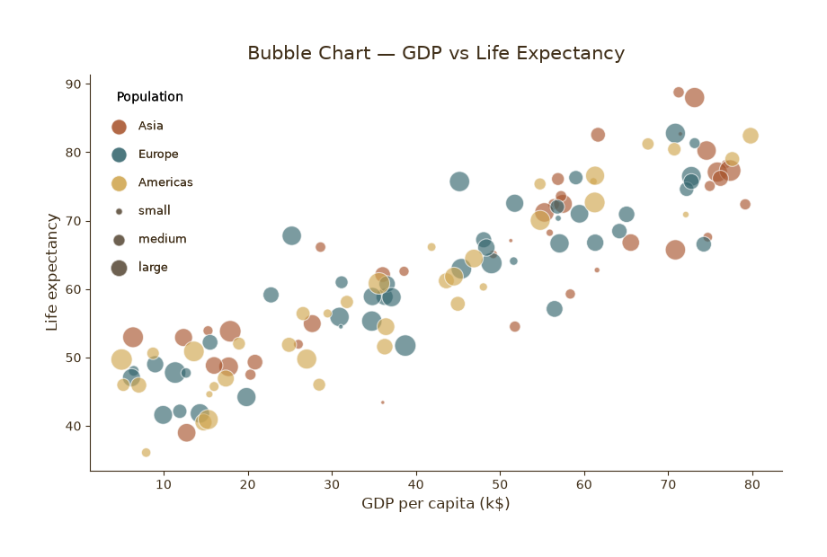
气泡图(大小 + 颜色双编码)
Python50 行
import matplotlib.pyplot as plt
import numpy as np

COLORS = ["#A8552E", "#35666E", "#D0A64F", "#3F2E18", "#7E8F52"]

np.random.seed(1)
n = 120
gdp = np.random.uniform(5, 80, n)          # x
life = 40 + 0.5 * gdp + np.random.normal(0, 6, n)   # y
pop = np.random.uniform(1, 100, n)         # 气泡大小

# 离散化为 3 个区域
regions = np.random.choice(["Asia", "Europe", "Americas"], n)
region_color = {"Asia": COLORS[0], "Europe": COLORS[1], "Americas": COLORS[2]}

fig, ax = plt.subplots(figsize=(8.5, 5.5))

for r, c in region_color.items():
    mask = regions == r
    ax.scatter(gdp[mask], life[mask],
               s=pop[mask] * 3,            # 大小映射
               color=c, edgecolor="white",
               linewidth=0.8, alpha=0.65, label=r)

# 图例:分别说明颜色和大小
ax.legend(frameon=False, fontsize=10, labelcolor=COLORS[3],
          loc="lower right", title="Region", title_fontsize=10)

# 手动加大小图例
for s_val, label in [(30, "small"), (90, "medium"), (180, "large")]:
    ax.scatter([], [], s=s_val, color=COLORS[3], alpha=0.5,
               edgecolor="white", label=label)
leg2 = ax.legend(frameon=False, fontsize=9, labelcolor=COLORS[3],
                 loc="upper left", title="Population", title_fontsize=10,
                 labelspacing=1.4, borderpad=1)
ax.add_artist(leg2)

ax.set_title("Bubble Chart — GDP vs Life Expectancy",
             fontsize=15, color=COLORS[3], pad=12)
ax.set_xlabel("GDP per capita (k$)", fontsize=12, color=COLORS[3])
ax.set_ylabel("Life expectancy", fontsize=12, color=COLORS[3])
ax.tick_params(axis="both", colors=COLORS[3])

for s in ("top", "right"):
    ax.spines[s].set_visible(False)
ax.spines["left"].set_color(COLORS[3])
ax.spines["bottom"].set_color(COLORS[3])

plt.tight_layout()
plt.show()带趋势线 + 边际分布
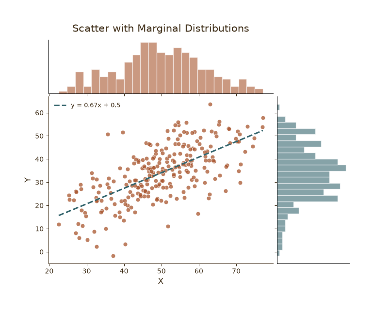
带趋势线 + 边际分布
Python53 行
import matplotlib.pyplot as plt
import numpy as np
from matplotlib.gridspec import GridSpec

COLORS = ["#A8552E", "#35666E", "#D0A64F", "#3F2E18", "#7E8F52"]

np.random.seed(7)
n = 250
x = np.random.normal(50, 12, n)
y = 0.7 * x + np.random.normal(0, 9, n)

fig = plt.figure(figsize=(8, 6))
gs = GridSpec(4, 4, figure=fig, hspace=0.05, wspace=0.05)

ax_main = fig.add_subplot(gs[1:, :-1])
ax_top  = fig.add_subplot(gs[0, :-1], sharex=ax_main)
ax_right = fig.add_subplot(gs[1:, -1], sharey=ax_main)

for a in (ax_main, ax_top, ax_right):
    a.tick_params(colors=COLORS[3])
    for s in ("top", "right"):
        a.spines[s].set_visible(False)
    ax_main.spines["left"].set_color(COLORS[3])
    ax_main.spines["bottom"].set_color(COLORS[3])

# 主散点
ax_main.scatter(x, y, s=40, color=COLORS[0],
                edgecolor="white", linewidth=0.6, alpha=0.75)

# 回归线
coef = np.polyfit(x, y, 1)
xs = np.linspace(x.min(), x.max(), 100)
ax_main.plot(xs, np.polyval(coef, xs),
             color=COLORS[1], linewidth=2.2, linestyle="--",
             label=f"y = {coef[0]:.2f}x + {coef[1]:.1f}")
ax_main.legend(frameon=False, fontsize=9, labelcolor=COLORS[3], loc="upper left")

# 边际直方图
ax_top.hist(x, bins=25, color=COLORS[0], alpha=0.6, edgecolor="white")
ax_right.hist(y, bins=25, orientation="horizontal",
              color=COLORS[1], alpha=0.6, edgecolor="white")

ax_top.tick_params(labelbottom=False)
ax_right.tick_params(labelleft=False)
ax_top.set_yticks([]); ax_right.set_xticks([])

ax_main.set_xlabel("X", fontsize=12, color=COLORS[3])
ax_main.set_ylabel("Y", fontsize=12, color=COLORS[3])
ax_top.set_title("Scatter with Marginal Distributions",
                 fontsize=15, color=COLORS[3], pad=12)

plt.tight_layout()
plt.show()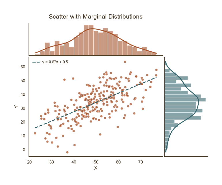
带趋势线 + 边际分布
Python72 行
import matplotlib.pyplot as plt
import numpy as np
from matplotlib.gridspec import GridSpec
from scipy.stats import gaussian_kde

COLORS = ["#A8552E", "#35666E", "#D0A64F", "#3F2E18", "#7E8F52"]

np.random.seed(7)
n = 250
x = np.random.normal(50, 12, n)
y = 0.7 * x + np.random.normal(0, 9, n)

fig = plt.figure(figsize=(8, 6))
gs = GridSpec(4, 4, figure=fig, hspace=0.05, wspace=0.05)

ax_main  = fig.add_subplot(gs[1:, :-1])
ax_top   = fig.add_subplot(gs[0, :-1], sharex=ax_main)
ax_right = fig.add_subplot(gs[1:, -1], sharey=ax_main)

for a in (ax_main, ax_top, ax_right):
    a.tick_params(colors=COLORS[3])
    for s in ("top", "right"):
        a.spines[s].set_visible(False)
    ax_main.spines["left"].set_color(COLORS[3])
    ax_main.spines["bottom"].set_color(COLORS[3])

# 主散点
ax_main.scatter(x, y, s=40, color=COLORS[0],
                edgecolor="white", linewidth=0.6, alpha=0.75)

# 回归线
coef = np.polyfit(x, y, 1)
xs = np.linspace(x.min(), x.max(), 100)
ax_main.plot(xs, np.polyval(coef, xs),
             color=COLORS[1], linewidth=2.2, linestyle="--",
             label=f"y = {coef[0]:.2f}x + {coef[1]:.1f}")
ax_main.legend(frameon=False, fontsize=9, labelcolor=COLORS[3], loc="upper left")

# ==================== 顶部:直方图 + KDE ====================
top_color = COLORS[0]   # 顶部主题色
ax_top.hist(x, bins=25, color=top_color, alpha=0.6,
            edgecolor="white", density=True)

kde_x = gaussian_kde(x)
grid_x = np.linspace(x.min(), x.max(), 300)
ax_top.plot(grid_x, kde_x(grid_x),
            color=top_color, linewidth=2.2)     # ← KDE 用主题色
# ==========================================================

# ==================== 右侧:横向直方图 + KDE ====================
right_color = COLORS[1]  # 右侧主题色
ax_right.hist(y, bins=25, orientation="horizontal",
              color=right_color, alpha=0.6,
              edgecolor="white", density=True)

kde_y = gaussian_kde(y)
grid_y = np.linspace(y.min(), y.max(), 300)
ax_right.plot(kde_y(grid_y), grid_y,
              color=right_color, linewidth=2.2)   # ← KDE 用主题色
# ============================================================

ax_top.tick_params(labelbottom=False)
ax_right.tick_params(labelleft=False)
ax_top.set_yticks([]); ax_right.set_xticks([])

ax_main.set_xlabel("X", fontsize=12, color=COLORS[3])
ax_main.set_ylabel("Y", fontsize=12, color=COLORS[3])
ax_top.set_title("Scatter with Marginal Distributions",
                 fontsize=15, color=COLORS[3], pad=12)

plt.tight_layout()
plt.show()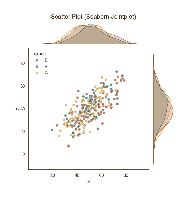
带趋势线 + 边际分布
Python42 行
import matplotlib.pyplot as plt
import seaborn as sns
import pandas as pd
import numpy as np

COLORS = ["#A8552E", "#35666E", "#D0A64F", "#3F2E18", "#7E8F52"]

sns.set_theme(style="white", rc={
    "axes.edgecolor": COLORS[3],
    "text.color": COLORS[3],
    "axes.labelcolor": COLORS[3],
    "xtick.color": COLORS[3],
    "ytick.color": COLORS[3],
})

np.random.seed(0)
n = 240
df = pd.DataFrame({
    "x": np.random.normal(50, 12, n),
    "group": np.random.choice(["A", "B", "C"], n),
})
df["y"] = 0.8 * df["x"] + np.random.normal(0, 8, n)

# 散点 + 回归线 + 边际分布
g = sns.jointplot(
    data=df, x="x", y="y", hue="group",
    palette=COLORS[:3],
    height=6, s=45, alpha=0.75,
    edgecolor="white", linewidth=0.6,
)
g.figure.suptitle("Scatter Plot (Seaborn Jointplot)",
                  fontsize=15, color=COLORS[3], y=1.02)

# ---- 关键修改:去掉图例边框并放到左上角 ----
legend = g.figure.legends[0] if g.figure.legends else g.ax_joint.get_legend()
legend.set_frame_on(False)          # 去掉边框
legend.get_frame().set_alpha(0)     # 同时让背景透明(可选)
legend.set_loc("upper left")        # 放到左上角
# ------------------------------------------

g.figure.savefig("scatter_seaborn.png", dpi=120, facecolor=BG)
plt.show()