2D DENSITYPLOT
绘图 · 第 6 / 36 章
KDE 二维密度图
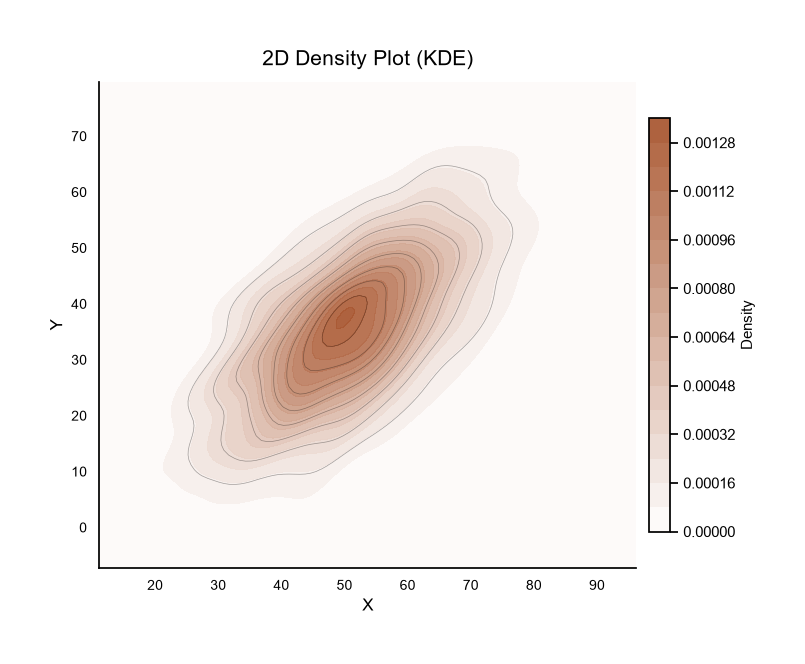
KDE 二维密度图
Python72 行
import matplotlib.pyplot as plt
import numpy as np
from scipy.stats import gaussian_kde
from matplotlib.colors import LinearSegmentedColormap

# 背景色(白)→ 主题色
BG = "#FFFFFF"
CMAP = LinearSegmentedColormap.from_list("theme", [BG, "#A8552E"], N=256)

BLACK = "#000000"   # 统一黑色

np.random.seed(42)
n = 2000
x = np.random.normal(50, 12, n)
y = 0.7 * x + np.random.normal(0, 10, n)

fig, ax = plt.subplots(figsize=(7.5, 6))

# ==================== 取消背景色 ====================
fig.patch.set_facecolor("white")   # 画布背景:白
ax.set_facecolor("white")          # 坐标区背景:白
# 若想完全透明(导出 PNG 时透出下层):
# fig.patch.set_alpha(0)
# ax.set_facecolor("none")
# ====================================================

# 计算二维 KDE
kde = gaussian_kde(np.vstack([x, y]))
xi, yi = np.mgrid[x.min():x.max():100j, y.min():y.max():100j]
zi = kde(np.vstack([xi.ravel(), yi.ravel()])).reshape(xi.shape)

# 填充等高线
cf = ax.contourf(xi, yi, zi, levels=20, cmap=CMAP, alpha=0.95)

# 叠加稀疏等高线
ax.contour(xi, yi, zi, levels=8, colors=BLACK,
           linewidths=0.5, alpha=0.35)

# 色条
cbar = fig.colorbar(cf, ax=ax, shrink=0.85, pad=0.02)
cbar.set_label("Density", fontsize=11, color=BLACK)
cbar.ax.tick_params(colors=BLACK)
cbar.outline.set_edgecolor(BLACK)

# 标题与标签:全部黑色
ax.set_title("2D Density Plot (KDE)", fontsize=15, color=BLACK, pad=12)
ax.set_xlabel("X", fontsize=12, color=BLACK)
ax.set_ylabel("Y", fontsize=12, color=BLACK)

# 刻度:黑色
ax.tick_params(axis="both",
               which="major",
               colors=BLACK,
               labelsize=10,
               direction="out",
               length=5,
               width=1.0)
ax.tick_params(axis="both",
               which="minor",
               colors=BLACK,
               direction="out",
               length=3,
               width=0.6)

# 边框
for s in ("top", "right"):
    ax.spines[s].set_visible(False)
ax.spines["left"].set_color(BLACK)
ax.spines["bottom"].set_color(BLACK)

plt.tight_layout()
plt.show()hexbin
当点数 >10000 时,hexbin 比 KDE 更快,且蜂窝结构边界清晰
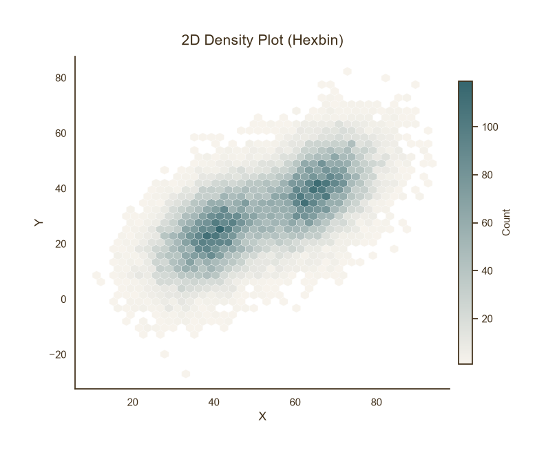
hexbin
Python41 行
import matplotlib.pyplot as plt
import numpy as np
from matplotlib.colors import LinearSegmentedColormap

CMAP = LinearSegmentedColormap.from_list("theme", [BG, "#35666E"], N=256)

np.random.seed(0)
n = 20000
# 双峰数据
x = np.concatenate([np.random.normal(40, 8, n//2),
                    np.random.normal(65, 8, n//2)])
y = 0.6 * x + np.random.normal(0, 10, n)

fig, ax = plt.subplots(figsize=(7.5, 6))

hb = ax.hexbin(
    x, y,
    gridsize=40,          # 蜂窝密度,越大越细
    cmap=CMAP,
    mincnt=1,             # 空网格不填色
    linewidths=0.2,
    edgecolors="white",
)

cbar = fig.colorbar(hb, ax=ax, shrink=0.85, pad=0.02)
cbar.set_label("Count", fontsize=11, color="#3F2E18")
cbar.ax.tick_params(colors="#3F2E18")
cbar.outline.set_edgecolor("#3F2E18")

ax.set_title("2D Density Plot (Hexbin)", fontsize=15, color="#3F2E18", pad=12)
ax.set_xlabel("X", fontsize=12, color="#3F2E18")
ax.set_ylabel("Y", fontsize=12, color="#3F2E18")
ax.tick_params(axis="both", colors="#3F2E18")

for s in ("top", "right"):
    ax.spines[s].set_visible(False)
ax.spines["left"].set_color("#3F2E18")
ax.spines["bottom"].set_color("#3F2E18")

plt.tight_layout()
plt.show()密度图 + 散点叠加
低密度区用散点展示原始观测,高密度区用密度填充,兼顾两者
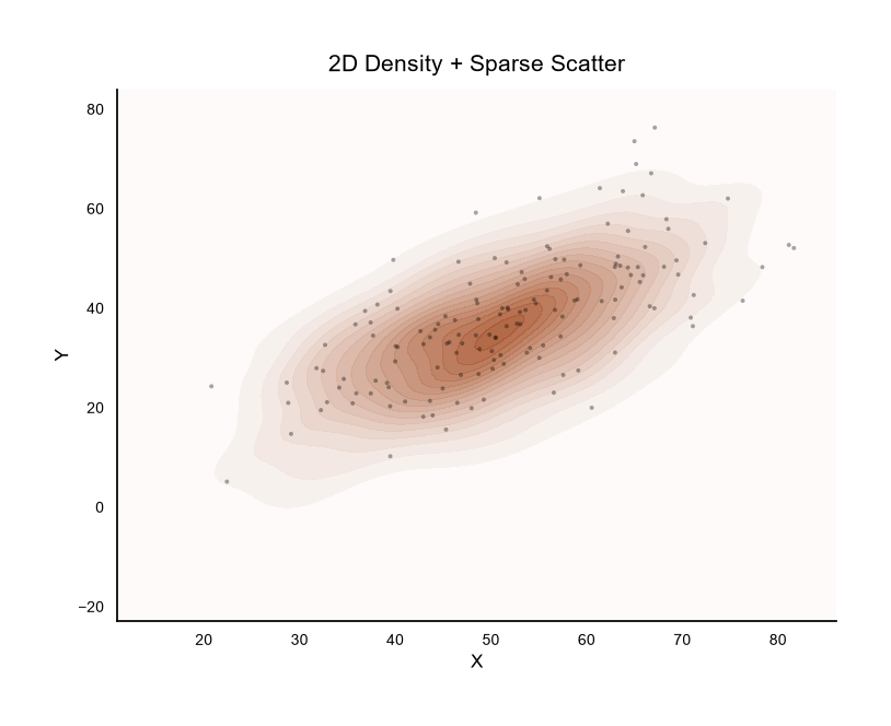
密度图 + 散点叠加
Python63 行
import matplotlib.pyplot as plt
import numpy as np
from scipy.stats import gaussian_kde
from matplotlib.colors import LinearSegmentedColormap

# 背景色改为白(取消原米色底)
BG = "#FFFFFF"
CMAP = LinearSegmentedColormap.from_list("theme", [BG, "#A8552E"], N=256)

BLACK = "#000000"

np.random.seed(7)
n = 1500
x = np.random.normal(50, 12, n)
y = 0.7 * x + np.random.normal(0, 10, n)

fig, ax = plt.subplots(figsize=(7.5, 6))

# ==================== 取消背景色 ====================
fig.patch.set_facecolor("white")   # 画布背景:白
ax.set_facecolor("white")          # 坐标区背景:白


# 底层:密度填充
kde = gaussian_kde(np.vstack([x, y]))
xi, yi = np.mgrid[x.min():x.max():100j, y.min():y.max():100j]
zi = kde(np.vstack([xi.ravel(), yi.ravel()])).reshape(xi.shape)
ax.contourf(xi, yi, zi, levels=20, cmap=CMAP, alpha=0.9)

# 上层:抽稀后的散点
idx = np.random.choice(n, size=n // 10, replace=False)
ax.scatter(x[idx], y[idx], s=8, color=BLACK,
           alpha=0.35, edgecolor="none", zorder=3)

# 标题与标签:全部黑色
ax.set_title("2D Density + Sparse Scatter",
             fontsize=15, color=BLACK, pad=12)
ax.set_xlabel("X", fontsize=12, color=BLACK)
ax.set_ylabel("Y", fontsize=12, color=BLACK)

# 刻度:黑色,并加上刻度线
ax.tick_params(axis="both",
               which="major",
               colors=BLACK,
               labelsize=10,
               direction="out",
               length=5,
               width=1.0)
ax.tick_params(axis="both",
               which="minor",
               colors=BLACK,
               direction="out",
               length=3,
               width=0.6)

# 边框
for s in ("top", "right"):
    ax.spines[s].set_visible(False)
ax.spines["left"].set_color(BLACK)
ax.spines["bottom"].set_color(BLACK)

plt.tight_layout()
plt.show()