PCA
绘图 · 第 15 / 36 章
基础 PCA 散点图
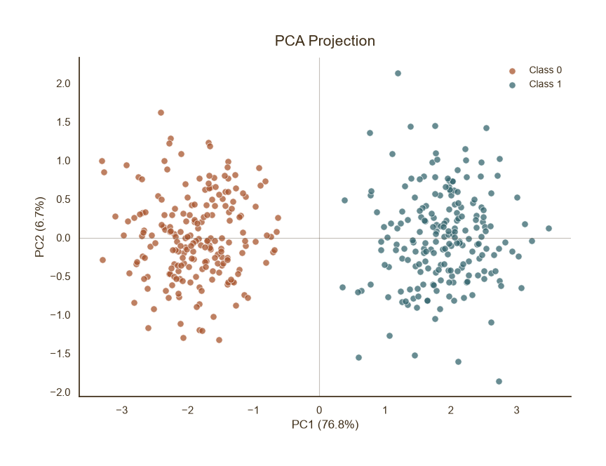
基础 PCA 散点图
Python52 行
import matplotlib.pyplot as plt
import numpy as np
from sklearn.decomposition import PCA
from sklearn.preprocessing import StandardScaler

COLORS = ["#A8552E", "#35666E", "#D0A64F", "#3F2E18", "#7E8F52"]
BG = "#F7F3EC"

np.random.seed(42)
# 模拟 5 维数据,两组分离
n = 200
X = np.vstack([
    np.random.normal(0, 1, (n, 5)),
    np.random.normal(3, 1, (n, 5)),
])
y = np.array([0] * n + [1] * n)

# 标准化 → PCA
X_scaled = StandardScaler().fit_transform(X)
pca = PCA(n_components=2)
X_pca = pca.fit_transform(X_scaled)

fig, ax = plt.subplots(figsize=(8, 6))

for label, c in zip([0, 1], [COLORS[0], COLORS[1]]):
    mask = y == label
    ax.scatter(X_pca[mask, 0], X_pca[mask, 1],
               s=45, color=c, edgecolor="white",
               linewidth=0.6, alpha=0.75,
               label=f"Class {label}")

# 坐标轴解释方差比例
ev = pca.explained_variance_ratio_ * 100
ax.set_xlabel(f"PC1 ({ev[0]:.1f}%)", fontsize=12, color=COLORS[3])
ax.set_ylabel(f"PC2 ({ev[1]:.1f}%)", fontsize=12, color=COLORS[3])

ax.set_title("PCA Projection", fontsize=15, color=COLORS[3], pad=12)
ax.tick_params(axis="both", colors=COLORS[3])
ax.legend(frameon=False, fontsize=10, labelcolor=COLORS[3],
          loc="upper right")

# 零参考线
ax.axhline(0, color=COLORS[3], linewidth=0.8, alpha=0.3)
ax.axvline(0, color=COLORS[3], linewidth=0.8, alpha=0.3)

for s in ("top", "right"):
    ax.spines[s].set_visible(False)
ax.spines["left"].set_color(COLORS[3])
ax.spines["bottom"].set_color(COLORS[3])

plt.tight_layout()
plt.show()带载荷向量
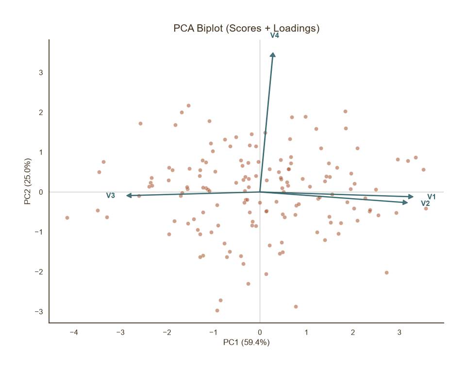
带载荷向量
Python61 行
import matplotlib.pyplot as plt
import numpy as np
from sklearn.decomposition import PCA
from sklearn.preprocessing import StandardScaler

COLORS = ["#A8552E", "#35666E", "#D0A64F", "#3F2E18", "#7E8F52"]
BG = "#F7F3EC"

np.random.seed(0)
n = 150
# 模拟 4 个变量:V1、V2 强相关,V3、V4 独立
X = np.random.normal(0, 1, (n, 4))
X[:, 1] = X[:, 0] * 0.8 + np.random.normal(0, 0.5, n)
X[:, 2] = -X[:, 0] * 0.5 + np.random.normal(0, 0.7, n)
feature_names = ["V1", "V2", "V3", "V4"]

X_scaled = StandardScaler().fit_transform(X)
pca = PCA(n_components=2)
X_pca = pca.fit_transform(X_scaled)
loadings = pca.components_.T * np.sqrt(pca.explained_variance_)

fig, ax = plt.subplots(figsize=(9, 7))

# 散点
ax.scatter(X_pca[:, 0], X_pca[:, 1],
           s=35, color=COLORS[0], edgecolor="white",
           linewidth=0.5, alpha=0.55)

# 载荷箭头
scale = 3.5   # 箭头缩放,视数据范围调整
for i, name in enumerate(feature_names):
    ax.arrow(0, 0,
             loadings[i, 0] * scale,
             loadings[i, 1] * scale,
             color=COLORS[1], width=0.015,
             head_width=0.12, head_length=0.10,
             length_includes_head=True,
             zorder=5, alpha=0.9)
    ax.text(loadings[i, 0] * scale * 1.12,
            loadings[i, 1] * scale * 1.12,
            name, fontsize=11, color=COLORS[1],
            ha="center", va="center", fontweight="bold")

ev = pca.explained_variance_ratio_ * 100
ax.set_xlabel(f"PC1 ({ev[0]:.1f}%)", fontsize=12, color=COLORS[3])
ax.set_ylabel(f"PC2 ({ev[1]:.1f}%)", fontsize=12, color=COLORS[3])

ax.set_title("PCA Biplot (Scores + Loadings)",
             fontsize=15, color=COLORS[3], pad=12)
ax.tick_params(axis="both", colors=COLORS[3])

ax.axhline(0, color=COLORS[3], linewidth=0.8, alpha=0.3)
ax.axvline(0, color=COLORS[3], linewidth=0.8, alpha=0.3)

for s in ("top", "right"):
    ax.spines[s].set_visible(False)
ax.spines["left"].set_color(COLORS[3])
ax.spines["bottom"].set_color(COLORS[3])

plt.tight_layout()
plt.show()带置信椭圆
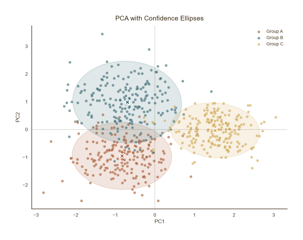
带置信椭圆
Python72 行
import matplotlib.pyplot as plt
import numpy as np
from sklearn.decomposition import PCA
from sklearn.preprocessing import StandardScaler
from matplotlib.patches import Ellipse
import matplotlib.transforms as transforms

COLORS = ["#A8552E", "#35666E", "#D0A64F", "#3F2E18", "#7E8F52"]
BG = "#F7F3EC"

def confidence_ellipse(x, y, ax, n_std=2.0, **kwargs):
    """绘制 2σ 置信椭圆。"""
    cov = np.cov(x, y)
    pearson = cov[0, 1] / np.sqrt(cov[0, 0] * cov[1, 1])
    ell_radius_x = np.sqrt(1 + pearson)
    ell_radius_y = np.sqrt(1 - pearson)
    ellipse = Ellipse((0, 0), width=ell_radius_x * 2,
                      height=ell_radius_y * 2, **kwargs)
    scale_x = np.sqrt(cov[0, 0]) * n_std
    scale_y = np.sqrt(cov[1, 1]) * n_std
    transf = (transforms.Affine2D()
              .rotate_deg(45)
              .scale(scale_x, scale_y)
              .translate(np.mean(x), np.mean(y)))
    ellipse.set_transform(transf + ax.transData)
    return ax.add_patch(ellipse)

np.random.seed(1)
n = 200
groups = {
    "Group A": np.random.normal([0, 0, 0], 1, (n, 3)),
    "Group B": np.random.normal([3, 1, 0], 1.2, (n, 3)),
    "Group C": np.random.normal([1, 4, 2], 0.8, (n, 3)),
}
X = np.vstack(list(groups.values()))
labels = np.repeat(list(groups.keys()), n)

X_scaled = StandardScaler().fit_transform(X)
X_pca = PCA(n_components=2).fit_transform(X_scaled)

fig, ax = plt.subplots(figsize=(9, 7))

for (name, _), c in zip(groups.items(), COLORS):
    mask = labels == name
    x, y = X_pca[mask, 0], X_pca[mask, 1]
    ax.scatter(x, y, s=40, color=c, edgecolor="white",
               linewidth=0.5, alpha=0.6, label=name)
    confidence_ellipse(x, y, ax, n_std=2.0,
                       facecolor=c, edgecolor=c,
                       alpha=0.15, linewidth=2.0)
    ax.scatter(x.mean(), y.mean(), s=120, color=c,
               edgecolor="white", linewidth=2.0,
               marker="X", zorder=5)

ax.set_title("PCA with Confidence Ellipses",
             fontsize=15, color=COLORS[3], pad=12)
ax.set_xlabel("PC1", fontsize=12, color=COLORS[3])
ax.set_ylabel("PC2", fontsize=12, color=COLORS[3])
ax.tick_params(axis="both", colors=COLORS[3])
ax.legend(frameon=False, fontsize=10, labelcolor=COLORS[3],
          loc="best")

ax.axhline(0, color=COLORS[3], linewidth=0.8, alpha=0.3)
ax.axvline(0, color=COLORS[3], linewidth=0.8, alpha=0.3)

for s in ("top", "right"):
    ax.spines[s].set_visible(False)
ax.spines["left"].set_color(COLORS[3])
ax.spines["bottom"].set_color(COLORS[3])

plt.tight_layout()
plt.show()Scree Plot
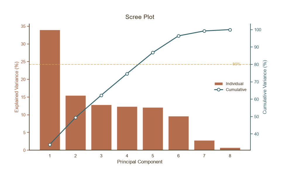
Scree Plot
Python65 行
import matplotlib.pyplot as plt
import numpy as np
from sklearn.decomposition import PCA
from sklearn.preprocessing import StandardScaler

COLORS = ["#A8552E", "#35666E", "#D0A64F", "#3F2E18", "#7E8F52"]
BG = "#F7F3EC"

np.random.seed(3)
# 8 维数据,前 3 个主成分占主导
X = np.random.normal(0, 1, (300, 8))
X[:, 1] = X[:, 0] * 0.9 + np.random.normal(0, 0.4, 300)
X[:, 2] = X[:, 0] * 0.7 + np.random.normal(0, 0.5, 300)

X_scaled = StandardScaler().fit_transform(X)
pca = PCA().fit(X_scaled)
ev = pca.explained_variance_ratio_ * 100
cum_ev = np.cumsum(ev)

fig, ax = plt.subplots(figsize=(9, 5.5))

x_pos = np.arange(1, len(ev) + 1)

# 柱状:单个主成分方差
bars = ax.bar(x_pos, ev, color=COLORS[0], alpha=0.85,
              edgecolor="white", linewidth=1.0,
              label="Individual")

# 折线:累积方差
ax2 = ax.twinx()
ax2.plot(x_pos, cum_ev, color=COLORS[1], linewidth=2.2,
         marker="o", markersize=7,
         markerfacecolor="white", markeredgecolor=COLORS[1],
         markeredgewidth=1.5, label="Cumulative")
ax2.axhline(80, color=COLORS[2], linestyle="--",
            linewidth=1.5, alpha=0.7)
ax2.text(len(ev) + 0.1, 80, "80%", fontsize=10,
         color=COLORS[2], va="center")

ax.set_xlabel("Principal Component", fontsize=12, color=COLORS[3])
ax.set_ylabel("Explained Variance (%)", fontsize=12, color=COLORS[0])
ax2.set_ylabel("Cumulative Variance (%)", fontsize=12, color=COLORS[1])
ax.tick_params(axis="y", colors=COLORS[0])
ax2.tick_params(axis="y", colors=COLORS[1])
ax.tick_params(axis="x", colors=COLORS[3])
ax.set_xticks(x_pos)

ax.set_title("Scree Plot", fontsize=15, color=COLORS[3], pad=12)

# 合并图例
lines1, labels1 = ax.get_legend_handles_labels()
lines2, labels2 = ax2.get_legend_handles_labels()
ax.legend(lines1 + lines2, labels1 + labels2,
          frameon=False, fontsize=10, labelcolor=COLORS[3],
          loc="center right")

for s in ("top",):
    ax.spines[s].set_visible(False)
    ax2.spines[s].set_visible(False)
ax.spines["left"].set_color(COLORS[0])
ax.spines["bottom"].set_color(COLORS[3])
ax2.spines["right"].set_color(COLORS[1])

plt.tight_layout()
plt.show()3D PCA 散点图
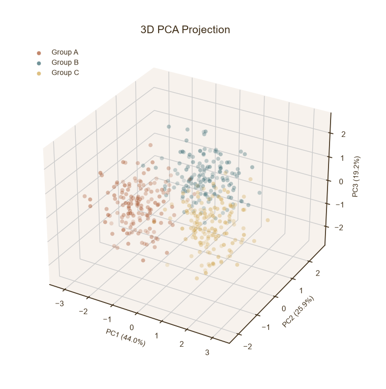
3D PCA 散点图
Python47 行
import matplotlib.pyplot as plt
import numpy as np
from sklearn.decomposition import PCA
from sklearn.preprocessing import StandardScaler

COLORS = ["#A8552E", "#35666E", "#D0A64F", "#3F2E18", "#7E8F52"]
BG = "#F7F3EC"

np.random.seed(4)
n = 150
groups = {
    "Group A": np.random.normal([0, 0, 0, 0], 1, (n, 4)),
    "Group B": np.random.normal([3, 2, 1, 0], 1, (n, 4)),
    "Group C": np.random.normal([1, 4, 2, 1], 1, (n, 4)),
}
X = np.vstack(list(groups.values()))
labels = np.repeat(list(groups.keys()), n)

X_scaled = StandardScaler().fit_transform(X)
pca = PCA(n_components=3)
X_pca = pca.fit_transform(X_scaled)
ev = pca.explained_variance_ratio_ * 100

fig = plt.figure(figsize=(9, 7))
ax = fig.add_subplot(111, projection="3d")

for (name, _), c in zip(groups.items(), COLORS):
    mask = labels == name
    ax.scatter(X_pca[mask, 0], X_pca[mask, 1], X_pca[mask, 2],
               s=35, color=c, edgecolor="white",
               linewidth=0.4, alpha=0.7, label=name)

ax.set_xlabel(f"PC1 ({ev[0]:.1f}%)", fontsize=10, color=COLORS[3])
ax.set_ylabel(f"PC2 ({ev[1]:.1f}%)", fontsize=10, color=COLORS[3])
ax.set_zlabel(f"PC3 ({ev[2]:.1f}%)", fontsize=10, color=COLORS[3])

ax.set_title("3D PCA Projection", fontsize=15,
             color=COLORS[3], pad=14)
ax.tick_params(axis="both", colors=COLORS[3])
ax.legend(frameon=False, fontsize=10, labelcolor=COLORS[3],
          loc="upper left")

for pane in (ax.xaxis, ax.yaxis, ax.zaxis):
    pane.set_pane_color((0.97, 0.95, 0.93, 1.0))

plt.tight_layout()
plt.show()