子图与布局

Matplotlib · 第 2 / 43 章

2026-10-121,055 字约 3 分钟

plt.subplots

创建画布 Figure，并在画布中创建一个或多个子图 Axes。

Python9 行

fig, ax = plt.subplots(
    nrows=1,                 # 子图的行数
    ncols=1,                 # 子图的列数
    figsize=None,            # 整张画布的尺寸，单位为英寸,如figsize=(10, 6)
    sharex=False,            # 是否共享 X 轴
    sharey=False,            # 是否共享 Y 轴
    squeeze=True,            # 是否压缩返回的 Axes 数组维度
    layout=None              # 自动布局设置
)

以下是各种示例：

Python2 行

import matplotlib.pyplot as plt
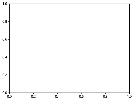
fig, ax = plt.subplots()

因为还没有在画布上绘制任何东西，运行上面这段代码后不会出现任何东西，以下只是示意图

Pasted image 20261010134435

Python1 行

fig, axs = plt.subplots(2, 3)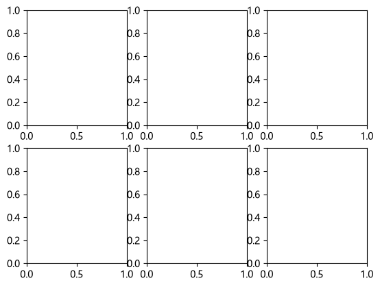

Pasted image 20261010134445

Python2 行

fig, ax = plt.subplots(2, 2, sharex=True, sharey=True)       # 所有子图共享轴
#sharex 和 sharey 除了 True/False，还支持 'row'、'col'、'all'、'none'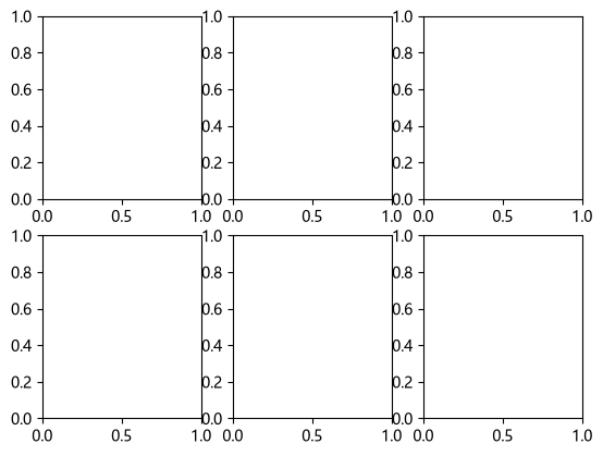

Pasted image 20261010134454

Python2 行

#同一行的子图共享 x 轴, 同一列的子图共享 y 轴。
fig, axs = plt.subplots(2, 2, sharex='row', sharey='col')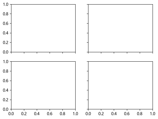

Pasted image 20261010134504

Python1 行

fig, axs = plt.subplots(2, 2, sharex='col', sharey='col')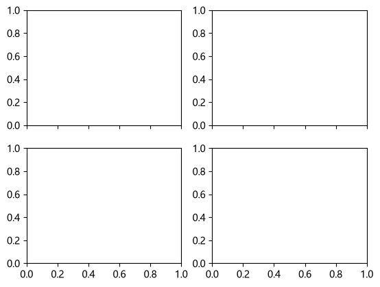

Pasted image 20261010134529

Python1 行

fig, axs = plt.subplots(1, 2, figsize=(10, 4), width_ratios=[2, 1])   # 列宽比 2:1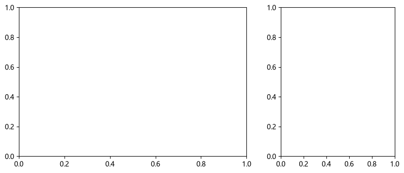

Pasted image 20261010134537

Python1 行

fig, axs = plt.subplots(2, 1, height_ratios=[3, 1])   # 行高比 3:1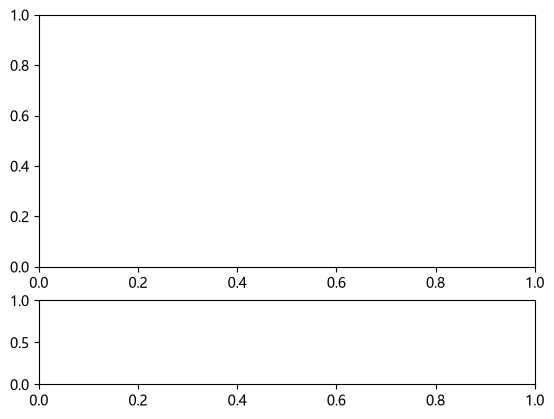

Pasted image 20261010134545

关于 squeeze 参数

squeeze 控制 plt.subplots() 返回的子图对象 axs 是否自动降维。默认 squeeze=True，Matplotlib 会移除长度为 1 的维度：

调用方式	`axs` 的返回形式
`plt.subplots(1, 1)`	单个 `Axes` 对象
`plt.subplots(1, 3)`	一维数组
`plt.subplots(3, 1)`	一维数组
`plt.subplots(2, 3)`	二维数组

设置 squeeze=False，则始终返回二维数组：

Python1 行

fig, axs = plt.subplots(2, 3, squeeze=False)

此时 axs.shape == (2, 3)，可以统一使用 axs[i, j] 访问子图。

编写需要适应不同子图行列数的通用函数时，使用 squeeze=False，确保索引方式始终一致，避免因返回维度变化而报错。

Python8 行

def plot_grid(nrows, ncols, data):
    fig, axs = plt.subplots(nrows, ncols, squeeze=False)

    for i in range(nrows):
        for j in range(ncols):
            axs[i, j].plot(data)

    return fig, axs

add_axes 与 add_subplot

当已经创建了 Figure，想手动添加子图时，可以使用add_subplot()和add_axes()，两者的区别在于定位方式。

Python8 行

import matplotlib.pyplot as plt

fig = plt.figure(figsize=(6, 4))
ax1 = fig.add_axes([0.0, 0.0, 0.6, 1.0])   # [左边界, 下边界, 宽, 高]，全是 0–1 的画布比例
ax2 = fig.add_axes([0.7, 0.2, 0.25, 0.5])

ax3 = fig.add_subplot(2, 2, 4)     # 用 GridSpec 定位，返回占满第 2×2 区域的 Axes
ax4 = fig.add_subplot(3, 1, (2, 2))# 占第 2 行整行（slice 语法）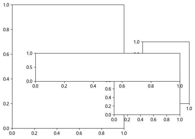

Pasted image 20261010134123

GridSpec：非均匀网格

Python19 行

import matplotlib.pyplot as plt
import numpy as np

fig = plt.figure(figsize=(8, 5))
gs = fig.add_gridspec(
    3, 3,                        # 在 fig 上创建一个 3 行 3 列的网格
    height_ratios=[1, 1, 0.5],   # 三行高度比为 1 : 1 : 0.5
    width_ratios=[1, 1, 0.6],    # 三列宽度比为 1 : 1 : 0.6
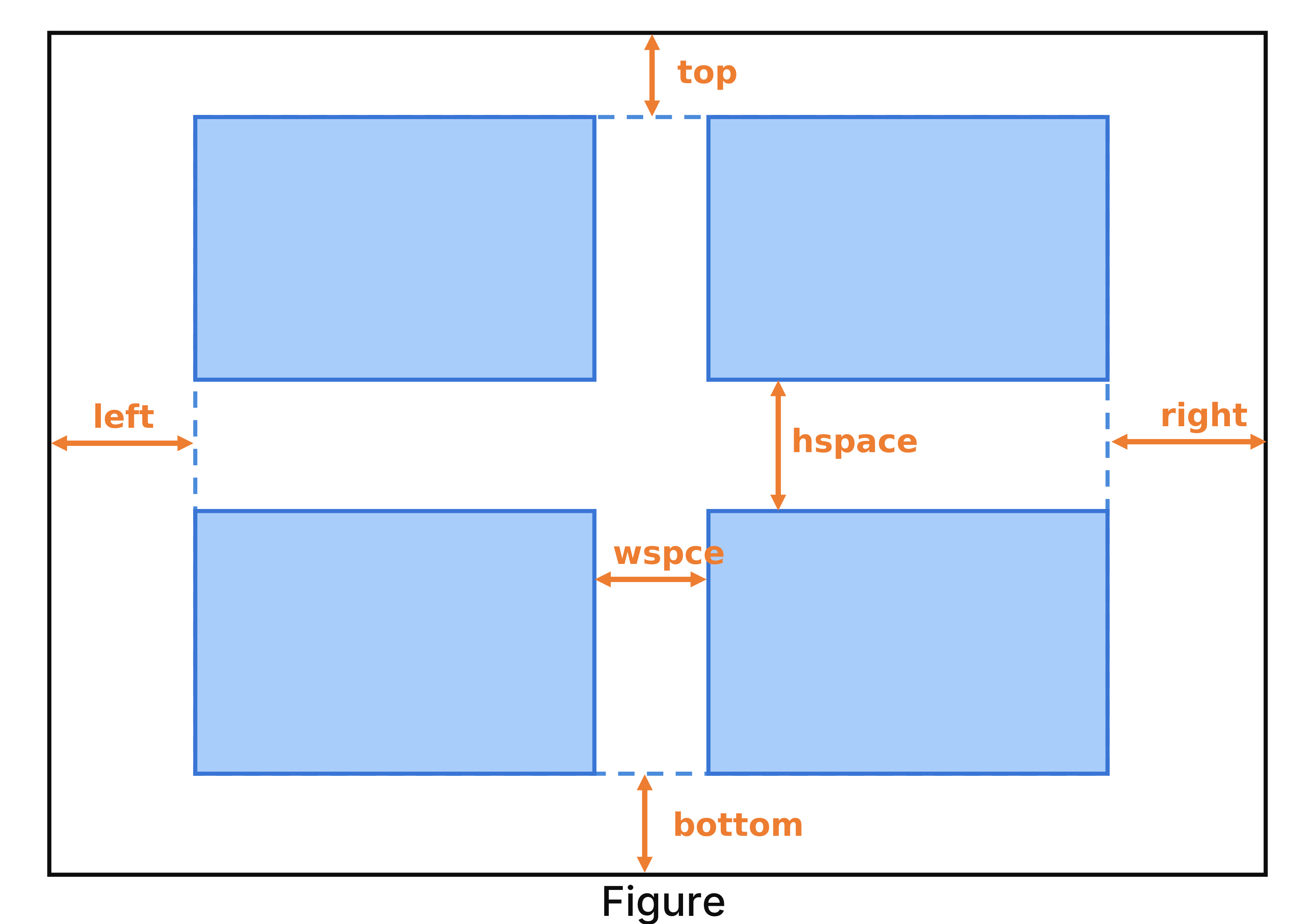
    hspace=0.4, wspace=0.3,      # 行间距，列间距
    left=.07, right=.97, top=.92, bottom=.08  #网格整体在画布中的边距
)

# 可视化布局情况
for i in range(3):
    for j in range(3):
        ax = fig.add_subplot(gs[i, j])
        ax.set_title(f'({i},{j})')

plt.show()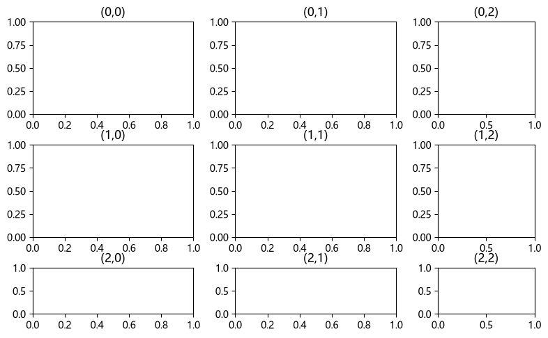

Pasted image 20261010133457

Python16 行

import matplotlib.pyplot as plt
import numpy as np

fig = plt.figure(figsize=(8, 5))
gs = fig.add_gridspec(
    3, 3,                        # 在 fig 上创建一个 3 行 3 列的网格
    height_ratios=[1, 1, 0.5],   # 三行高度比为 1 : 1 : 0.5
    width_ratios=[1, 1, 0.6],    # 三列宽度比为 1 : 1 : 0.6
    hspace=0.4, wspace=0.3,      # 行间距，列间距
    left=.07, right=.97, top=.92, bottom=.08  #网格整体在画布中的边距
)

ax_a = fig.add_subplot(gs[0, 0:2])      # 第 0 行，第 0~1 列，跨两列
ax_b = fig.add_subplot(gs[0, 2])        # 第 0 行，第 2 列
ax_c = fig.add_subplot(gs[1, :])        # 第 1 行，所有列
ax_d = fig.add_subplot(gs[2, 0:3])      # 第 2 行，所有列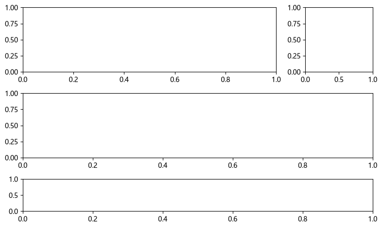

Pasted image 20261010133551

Python20 行

import matplotlib.pyplot as plt
import numpy as np                

fig = plt.figure(figsize=(8, 5))
gs = fig.add_gridspec(
    3, 3,
    height_ratios=[1, 1, 0.5],
    width_ratios=[1, 1, 0.6],
    hspace=0.4, wspace=0.3,
    left=.07, right=.97, top=.92, bottom=.08
)

ax_a = fig.add_subplot(gs[0, 0:2])
ax_b = fig.add_subplot(gs[0, 2])
ax_c = fig.add_subplot(gs[1, :])
ax_d = fig.add_subplot(gs[2, 0:3])

gs2 = fig.add_gridspec(1, 2, width_ratios=[1, 1], wspace=0.05)
ax_e = fig.add_subplot(gs2[0])
ax_f = fig.add_subplot(gs2[1], sharey=ax_e)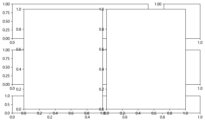

Pasted image 20261010133631

subplot_mosaic

subplot_mosaic：直接用字符画布局，最直观的新写法。

Python7 行

import matplotlib.pyplot as plt

# 传入的是一个二维列表，每个字符串代表一个格子。相同名字的格子会合并成一个 Axes
fig, axd = plt.subplot_mosaic([['left', 'top'], ['left', 'right']],
                              figsize=(6, 4), layout='constrained')
for name, ax in axd.items():
    ax.set_title(name)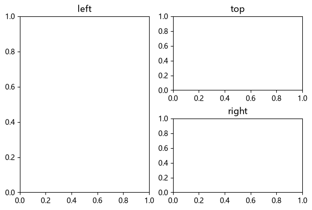

Pasted image 20261010123237

Python3 行

# 同一张网格里多种跨度的混排
fig, axd = plt.subplot_mosaic([['A', 'A', 'B'], ['C', 'D', 'B']],
                              height_ratios=[2, 1])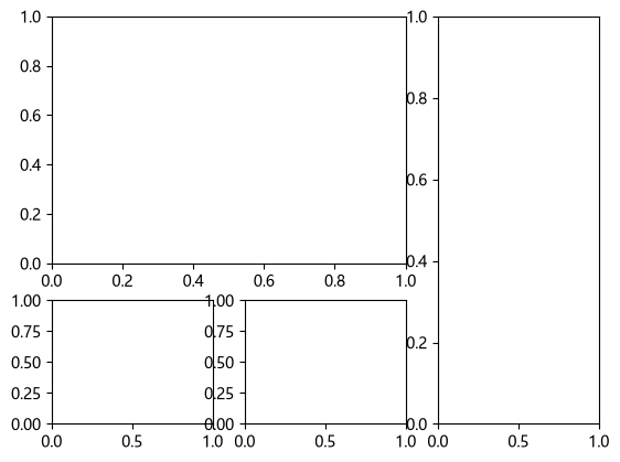

Pasted image 20261010123356

Python5 行

# subplot_mosaic 没有 squeeze 参数（返回的始终是 dict）；多余 kwarg 会透传给 Figure 而报错
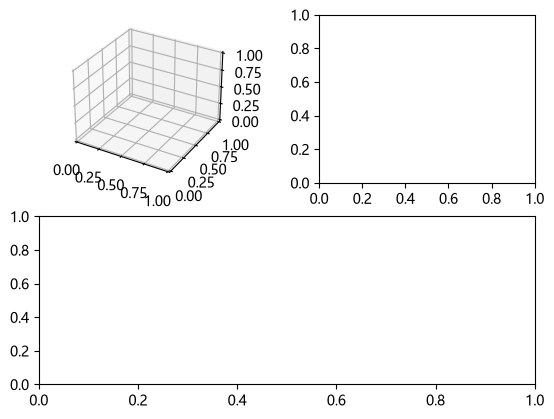
# 也可以给不同的格子不同的投影/设置
fig, axd = plt.subplot_mosaic([['A', 'B'], ['C', 'C']],
                              gridspec_kw={'wspace': .3}, #列与列之间的水平间距等于平均列宽的 30%
                              per_subplot_kw={'A': {'projection': '3d'}})

字符含义：S 必须出现且可重复（同一格拆成多个子区），数字 123 表示第 n 格（需 empty_sentinel=None），. 或 'None' 表示留空。 Pasted image 20261010123430

Python2 行

import matplotlib.pyplot as plt
fig, axs = plt.subplots(1, 2, subplot_kw={'projection': 'polar'})     # 极坐标子图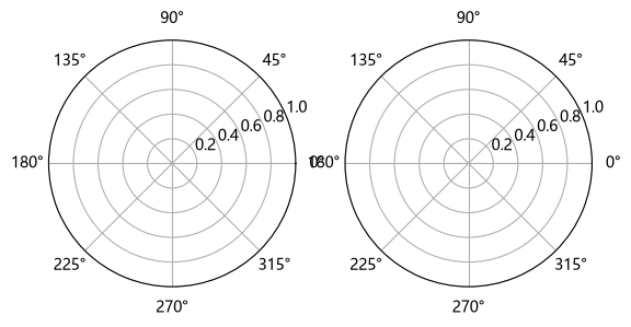

Pasted image 20261010132314

Python1 行

fig = plt.figure(); ax3d = fig.add_subplot(projection='3d')          # 3D 子图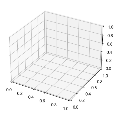

Pasted image 20261010132348

inset：图内嵌图

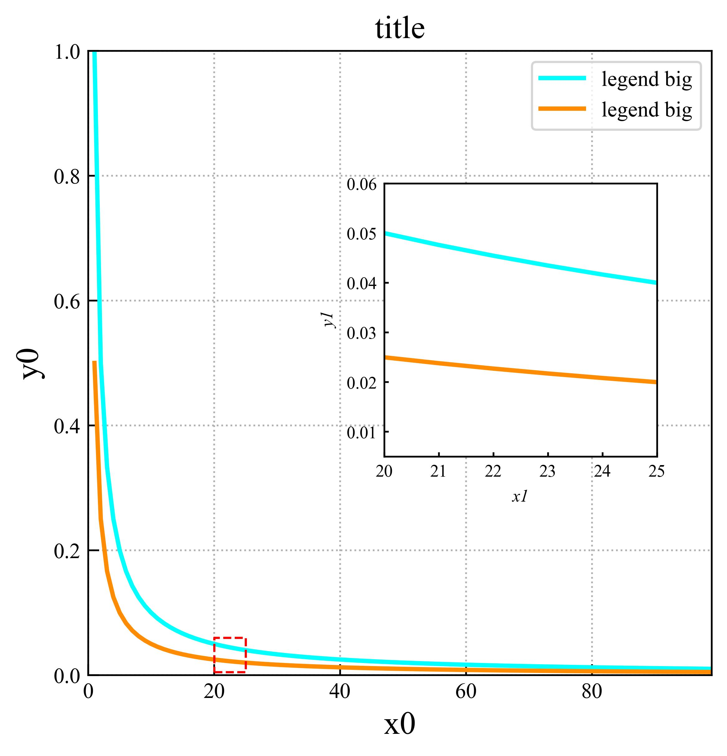
inset（嵌入图、插图），指的是在一张主图内部再放置一个较小的绘图区域。它常用于局部放大、展示数据细节、比较不同区域，或者在主图中补充直方图等辅助信息。

点我打开示例图片

区分三个概念：

Figure：整张画布。
主 Axes：主要绘图区域。
Inset Axes：嵌入在主图内部的小绘图区域。

Inset 并不是把一张已经生成的图片简单贴到主图上，而是创建一个独立的 Axes，因此它可以有自己的数据、坐标范围、刻度、标题和图例。

点我查看示例

Python17 行

import numpy as np
import matplotlib.pyplot as plt

x = np.linspace(0, 10, 300)
y = np.sin(x)

fig, ax = plt.subplots(figsize=(8, 5))

# 主图
ax.plot(x, y)
ax.set_title("Main Plot")

# 图内嵌图
axins = ax.inset_axes([0.55, 0.55, 0.35, 0.3])
axins.plot(x, y, color="red")

plt.show()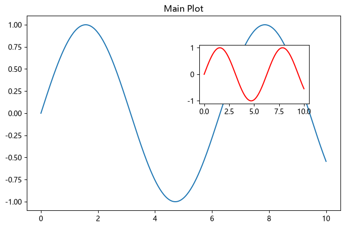

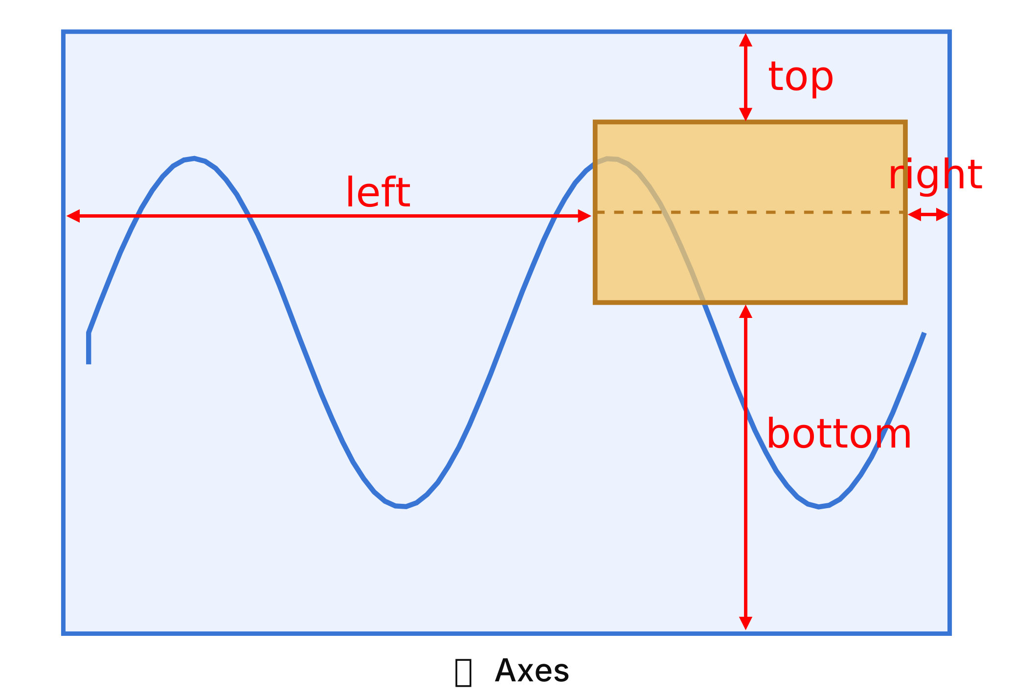
关键语句为 (值是相对于主 Axes 绘图区的比例，而不是整个 Figure 的比例)：

Python1 行

axins = ax.inset_axes([left, bottom, width, height])

这里的 ax.inset_axes() 与 fig.add_axes() 不同。前者通常相对于主 Axes 定位，后者默认相对于 Figure 定位。

除了 ax.inset_axes()，Matplotlib 还提供了：

Python1 行

from mpl_toolkits.axes_grid1.inset_locator import inset_axes

这个函数可以创建相对于主 Axes 定位的嵌入图，并允许使用英寸、百分比等方式指定大小。

点我查看示例

Python22 行

import numpy as np
import matplotlib.pyplot as plt
from mpl_toolkits.axes_grid1.inset_locator import inset_axes

x = np.linspace(0, 10, 200)
y = np.sin(x)

fig, ax = plt.subplots(figsize=(8, 5))
ax.plot(x, y)

axins = inset_axes(
    ax,
    width="35%",
    height="35%",
    loc="upper right"
)

axins.plot(x, y, color="red")
axins.set_xlim(4, 5)
axins.set_ylim(-1, 0)

plt.show()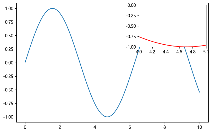

双 Y 轴 / 副坐标轴

双 Y 轴（双纵坐标轴）是指在同一张图中，使用两个不同的纵坐标轴展示两组数据。它特别适合比较量纲不同、数值范围差异较大，但横坐标相同的数据。创建双 Y 轴最常用的方法是：

Python2 行

fig, ax1 = plt.subplots()
ax2 = ax1.twinx()

它会创建一个新的 Axes 对象 ax2，使它与 ax1 共享 X 轴，但拥有独立的 Y 轴。

查看示例

Python45 行

import numpy as np
import matplotlib.pyplot as plt

# 模拟数据
months = np.arange(1, 13)
sales = [20, 25, 28, 35, 40, 45, 50, 48, 42, 38, 30, 25]
temperature = [3, 5, 10, 16, 22, 27, 30, 29, 24, 17, 10, 5]

# 创建画布和主坐标轴
fig, ax1 = plt.subplots(figsize=(9, 5))

# 左侧 Y 轴：销售额
line1, = ax1.plot(
    months, sales,
    color="tab:blue", marker="o",
    label="Sales"
)
ax1.set_xlabel("Month")
ax1.set_ylabel("Sales (10,000 yuan)", color="tab:blue")
ax1.tick_params(axis="y", labelcolor="tab:blue")

# 创建副坐标轴，共享 X 轴
ax2 = ax1.twinx()

# 右侧 Y 轴：气温
line2, = ax2.plot(
    months, temperature,
    color="tab:red", marker="s",
    label="Temperature"
)
ax2.set_ylabel("Temperature (°C)", color="tab:red")
ax2.tick_params(axis="y", labelcolor="tab:red")

# 设置标题
ax1.set_title("Monthly Sales and Temperature")

# 合并两个坐标轴的图例
ax1.legend(
    [line1, line2],
    [line1.get_label(), line2.get_label()],
    loc="upper left"
)

fig.tight_layout()
plt.show()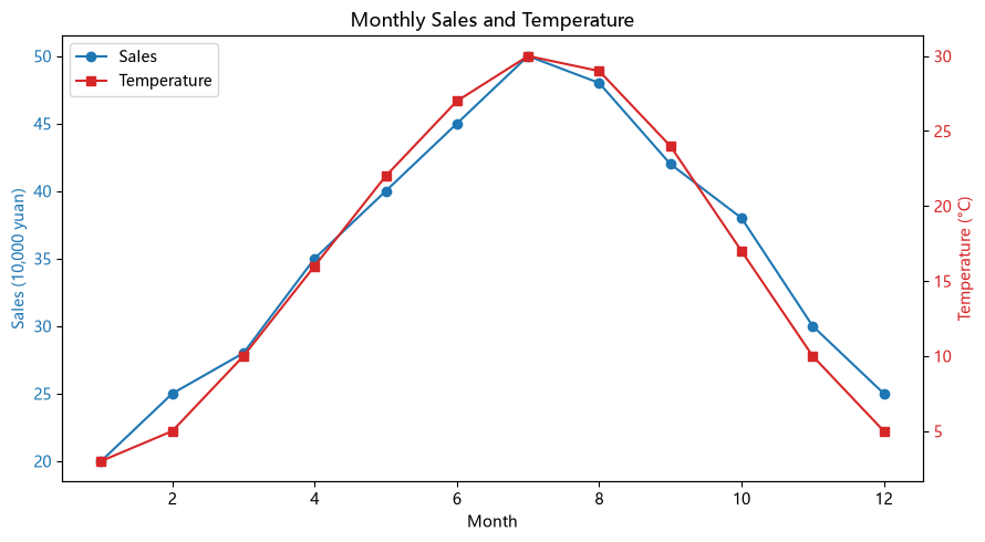

twinx() 返回的是另一个 Axes，而不是在原有 Axes 上简单增加一条右侧刻度。因此可以分别调用 ax1.plot() 和 ax2.plot()，也可以分别设置它们的 Y 轴范围。

还有一个与之对应的方法：twiny()。

方法	共享的轴	新增的轴	典型用途
`ax.twinx()`	X 轴	右侧 Y 轴	两组数据共用横坐标
`ax.twiny()`	Y 轴	顶部 X 轴	两组数据共用纵坐标

Python2 行

fig, ax1 = plt.subplots()
ax2 = ax1.twiny()

布局引擎

布局引擎主要解决一个问题：如何安排 Figure 中各个 Axes 的位置和大小，使标题、坐标轴标签、刻度、图例等元素尽可能不发生重叠或被裁切。

最常用的是：

layout="constrained"：创建 Figure 时启用布局引擎。
layout="tight"：使用紧凑布局引擎。
fig.tight_layout()：执行一次紧凑布局调整。这是一个方法，不是布局引擎本身。此外，layout=None 表示默认的布局行为;

常规绘图与多子图

Python1 行

fig, axes = plt.subplots(2, 2, layout="constrained")

一次性紧凑调整

Python2 行

fig, axes = plt.subplots(2, 2)
fig.tight_layout()

保存图片时裁切外围空白

Python1 行

fig.savefig("figure.png", bbox_inches="tight", dpi=300)

如果自动布局无法达到想要的效果，fig.subplots_adjust() 可以手动控制子图边距和间距可以直接控制 Figure 的边距和子图间距。

Python8 行

fig.subplots_adjust(
    left=0.12,
    right=0.95,
    bottom=0.12,
    top=0.90,
    wspace=0.30,
    hspace=0.35
)

这里的数值表示绘图区域边界在 Figure 中的相对位置。例如 left=0.1 表示绘图区域左边界位于画布宽度的 10% 处。