目录7
文章Matplotlib第 17 章
区间填充
Matplotlib · 第 17 / 43 章
fill_between() —— 两条水平曲线之间的填充带
fill() 要你自己写顶点,fill_between() 只要给两条曲线的 y 值。误差带、置信区间、阈值超标区间这三件事基本都用它。
Python10 行
Axes.fill_between(
    x,                  # 横坐标数组
    y1,                 # 一条边界
    y2=0,               # 另一条边界;默认 0
    where=None,         # 布尔掩码,只在 True 处填充
    interpolate=False,  # 是否插值到精确交点
    step=None,          # 阶梯填充:'pre' / 'post' / 'mid'
    data=None,
    **kwargs            # PolyCollection 属性
)| 参数 | 一句话 | 默认值的影响 |
|---|---|---|
y2 |
另一条边界 | 0——只给 y1 就是「与 x 轴之间」 |
where |
填充区域的掩码 | None 全填;给 bool 数组就只填一部分 |
interpolate |
边界是否插值到交点 | False,边缘是生硬的垂直截断 |
step |
阶梯填充 | None;与 step() 的 where 同义 |
alpha |
透明度 | 填充带一般 0.2~0.4 |
y2:默认是 0
Python11 行
import numpy as np
import matplotlib.pyplot as plt

x = np.linspace(0, 10, 300)
y = np.sin(x)

fig, ax = plt.subplots()
ax.plot(x, y, color='C0')
ax.plot(x, y + 0.6, color='C0')
ax.fill_between(x, y, y + 0.6, color='C0', alpha=0.3)
plt.show()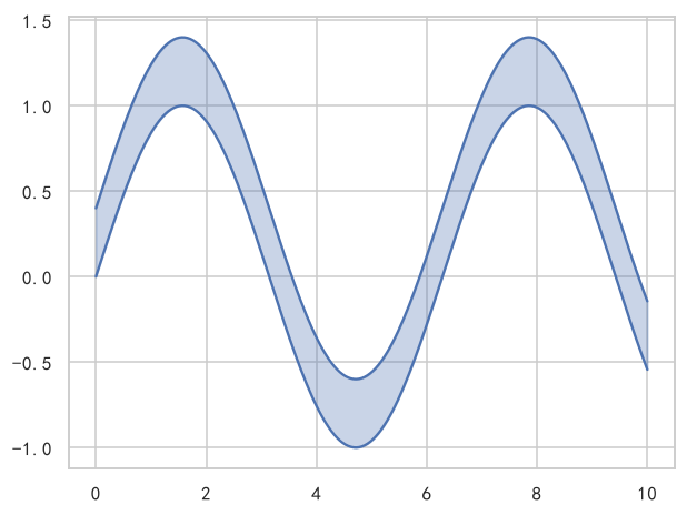
只传 y1 时,第二条边界是 y = 0——所以 fill_between(x, y) 就是「曲线与横轴围成的面积」。负值部分会填到轴下方,不会自动取绝对值,也不会报错。
Python4 行
ax.fill_between(x, y)             # 与 y=0 之间(正负分别填)
ax.fill_between(x, y, 0.2)        # 与水平线 y=0.2 之间
ax.fill_between(x, y, y + 0.6)    # 两条曲线之间
ax.fill_between(x, y * 0.9, y * 1.1)   # 相对误差带
where + interpolate:只填一部分
Python5 行
xc = np.linspace(0, 10, 11)        # ★ 采样点故意稀疏,才看得出差别
yc = np.sin(xc)

ax.fill_between(xc, yc, where=yc > 0, interpolate=False)   # 只在采样点为正处填
ax.fill_between(xc, yc, where=yc > 0, interpolate=True)    # 一直填到真正的零点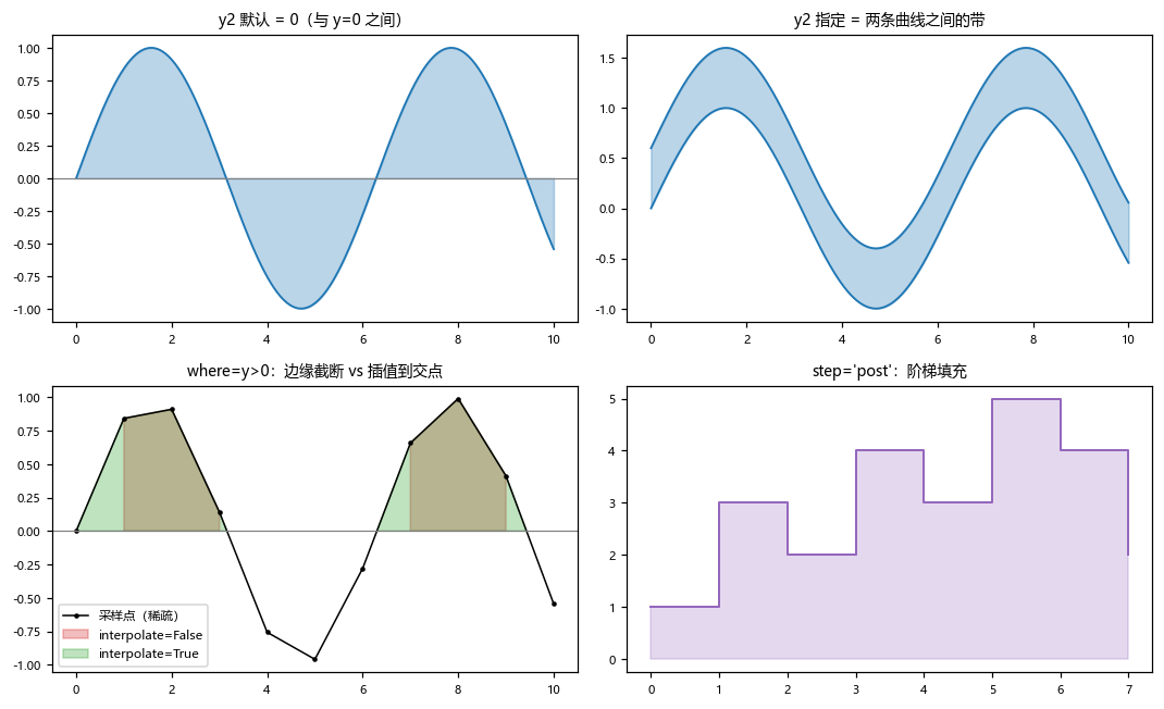
差异只在边界附近,而且采样越稀疏越明显:interpolate=False 时填充边缘是一条竖直线,落在最后一个满足条件的采样点上;interpolate=True 时才延伸到两条线的真实交点。
这也是个验证陷阱——如果你用 300 个点的 linspace 去对比 interpolate 开关,看到的两张图几乎完全一样,容易误判成「这个参数没用」。要看清差别必须用稀疏采样点。
step:阶梯填充
Python4 行
xs = np.arange(8)
ys = np.array([1, 3, 2, 4, 3, 5, 4, 2])
ax.step(xs, ys, where="post")
ax.fill_between(xs, ys, step="post", alpha=0.25)
step="post" 与 step() 的 where="post" 是同一套语义。填充和台阶必须用同一个值,否则错半格。
典型用法:均值 ± 标准差置信带
Python5 行
mean = 3 + 1.2 * np.sin(x / 2)
std = 0.35 + 0.15 * np.cos(x / 1.5)

ax.plot(x, mean, color="C0")
ax.fill_between(x, mean - std, mean + std, color="C0", alpha=0.25)
这是科研图里出现频率最高的三行代码。注意 alpha 别超过 0.4,否则压住下面的网格线和曲线。
返回对象
Python12 行
lo, hi = np.sin(x) - 0.3, np.sin(x) + 0.3
coll = ax.fill_between(x, lo, hi)
print(type(coll).__name__)
# 输出: FillBetweenPolyCollection

print(hasattr(coll, "get_paths"))
# 输出: True

coll.set_alpha(0.5)
coll.set_color("#DD8452")
coll.set_zorder(1)                 # 填充带一般压在线下面
plt.show()3.10 起返回的是 FillBetweenPolyCollection(旧版是 PolyCollection)。它一个对象管整条带,不能像 fill 那样逐多边形取;要分段填就必须自己用 where 调用多次。
注意事项
y2默认0,不是「另一条曲线的自动推断」。where的掩码长度必须等于x,否则报ValueError。interpolate的差异在稀疏采样下才看得见,别用密采样去验证它。- 负值区间不会被「翻转」成面积,
fill_between(x, y)会填到轴下方。 - 3.10 的返回类型是
FillBetweenPolyCollection,旧代码里isinstance(coll, PolyCollection)的判断会失配。 - 多层叠加时把
alpha调到 0.15~0.25,否则颜色叠加后完全看不清结构。
综合示例:置信带 / 超标区间 / 阶梯填充
Python44 行
import numpy as np
import matplotlib.pyplot as plt

plt.rcParams["font.sans-serif"] = ["SimHei", "Microsoft YaHei", "DejaVu Sans"]
plt.rcParams["axes.unicode_minus"] = False

rng = np.random.default_rng(8)
x = np.linspace(0, 12, 200)
mean = 3 + 1.2 * np.sin(x / 2)
std = 0.35 + 0.15 * np.cos(x / 1.5)

fig, axes = plt.subplots(1, 3, figsize=(15, 4.2))

# ---- (a) 均值 ± 2 倍标准差 ----
axes[0].plot(x, mean, color="#1f77b4", linewidth=1.6, label="均值")
axes[0].fill_between(x, mean - 2 * std, mean + 2 * std,
                     color="#1f77b4", alpha=0.20, label="±2σ")
axes[0].fill_between(x, mean - std, mean + std,
                     color="#1f77b4", alpha=0.30, label="±1σ")
axes[0].legend(fontsize=8)
axes[0].set_title("(a) 双层置信带")

# ---- (b) 超标区间:where 掩码 + 阈值线 ----
thr = 3.9
axes[1].plot(x, mean, color="#333333", linewidth=1.4)
axes[1].axhline(thr, color="#C44E52", linestyle="--", linewidth=1.2)
axes[1].fill_between(x, mean, thr, where=mean > thr,
                     interpolate=True, color="#C44E52", alpha=0.35)
axes[1].set_title("(b) 超阈值区间(where + interpolate)")

# ---- (c) 阶梯填充:每日库存 vs 安全线 ----
days = np.arange(1, 13)
stock = np.array([120, 98, 85, 76, 90, 110, 130, 125, 95, 70, 88, 105])
axes[2].step(days, stock, where="post", color="#55A868", linewidth=1.6)
axes[2].axhline(80, color="gray", linestyle=":", linewidth=1.1)
axes[2].fill_between(days, stock, 80, step="post",
                     where=stock < 80, interpolate=True,
                     color="#C44E52", alpha=0.35)
axes[2].set_xlabel("日")
axes[2].set_ylabel("库存")
axes[2].set_title("(c) 低于安全线的日子(阶梯 + where)")

plt.tight_layout()
plt.show()(b) 和 (c) 是同一个套路:把掩码交给 where,把临界值作为 y2,就自动得到「超过阈值的那些片段」。