目录6
文章Matplotlib第 18 章
堆叠面积图
Matplotlib · 第 18 / 43 章
stackplot() —— 堆叠面积图
堆叠面积图同时回答两个问题:总量怎么变(外轮廓)和各成分占比怎么变(层厚)。它和 bar 堆叠图的区别是 x 轴连续——所以只适合时间序列。
Python9 行
Axes.stackplot(
    x,                 # 横坐标(连续,如日期或年份)
    *args,             # 各层的 y 序列:一个序列一层,可以给任意多层
    labels=(),         # 图例标签,长度必须等于层数
    colors=None,       # 各层颜色,列表
    baseline="zero",   # ★ 基线算法:zero / sym / wiggle / weighted_wiggle
    data=None,
    **kwargs           # alpha / hatch / edgecolor / linewidth
)| 参数 | 一句话 | 默认值的影响 |
|---|---|---|
*args |
各层的 y | 一序列一层;第一层贴基线 |
labels |
图例名 | 空元组,必须自己给才能 legend() |
colors |
各层颜色 | 不给就走 prop_cycle |
baseline |
基线算法 | "zero":全部从 0 往上堆 |
hatch |
各层花纹 | 可传列表,长度 = 层数 |
edgecolor |
层间描边 | 白色细线最有「分层」感 |
labels / colors:必须和层一一对应
Python18 行
import numpy as np
import matplotlib.pyplot as plt

x = np.arange(0, 10, 1)
y1 = np.array([1, 2, 3, 4, 5, 4, 3, 2, 1, 2])
y2 = np.array([2, 3, 2, 3, 2, 3, 2, 3, 2, 3])
y3 = np.array([1, 1, 2, 2, 3, 3, 2, 2, 1, 1])

fig, ax = plt.subplots()
ax.stackplot(x, y1, y2, y3,
             labels=['A', 'B', 'C'],
             colors=['#4C72B0', '#DD8452', '#55A868'],
             alpha=0.85)
ax.legend(loc='upper left')
ax.set_title("stackplot 基本示例")
ax.set_xlabel("时间")
ax.set_ylabel("总量")
plt.show()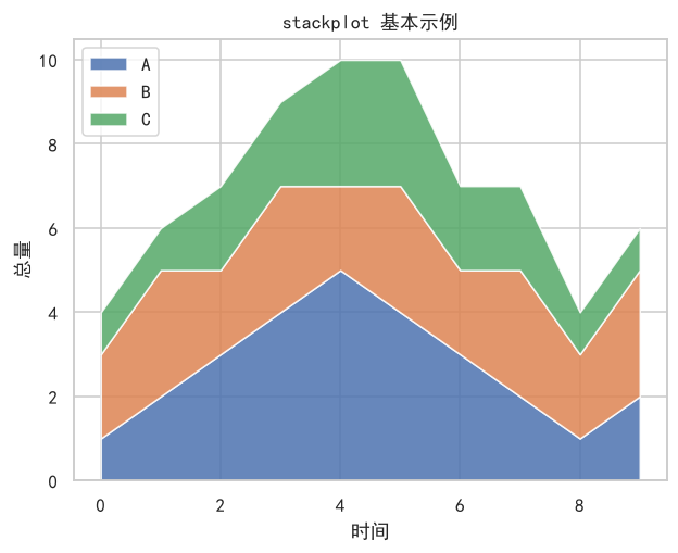
注意 labels 是元组/列表,一个字符串会被拆成字符逐个当标签。层数和 labels 长度不一致时不会报错,但图例会错位——这类静默错误最费时间。
baseline:四套堆叠算法
Python4 行
ax.stackplot(x, y1, y2, y3, baseline="zero")            # 默认:全部从 0 向上堆
ax.stackplot(x, y1, y2, y3, baseline="sym")             # 以 0 为中心对称堆叠
ax.stackplot(x, y1, y2, y3, baseline="wiggle")          # 让层厚变化最小
ax.stackplot(x, y1, y2, y3, baseline="weighted_wiggle") # 加权版 wiggle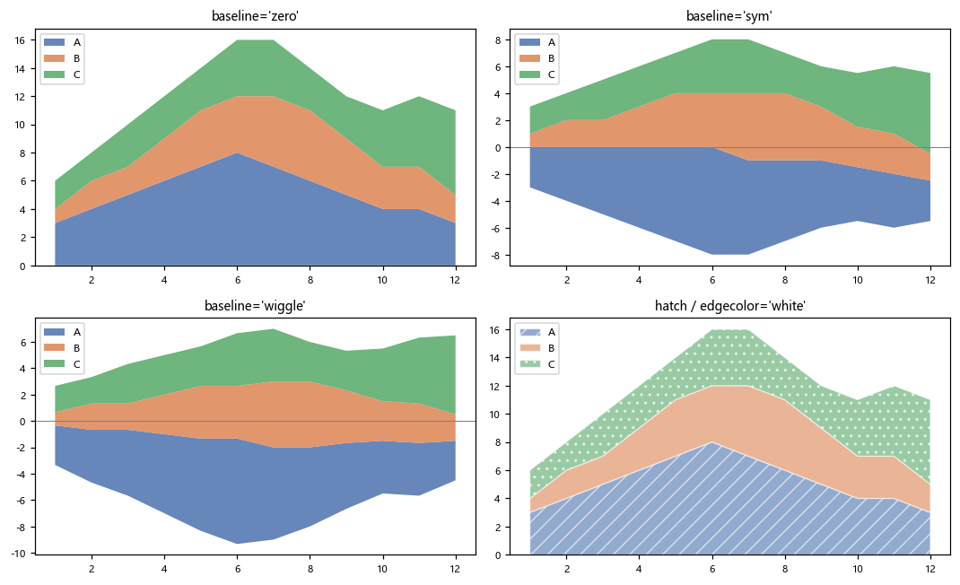
"zero":最常用。外轮廓 = 总和,每层从下往上累加。"sym":把总和平均摊到 0 上下两侧,看起来像双色流图,适合强调「有正有负」。"wiggle":按累积和的最小梯度排布基线,层厚看起来最平滑。适合只看构成比例、不关心绝对量时。"weighted_wiggle":wiggle 的加权版,层越厚权重越大,视觉效果更稳。
"sym" 和 "wiggle" 在数据平滑、层数少时几乎看不出差别——它们真正拉开差距是在层多、量级差异大的时候。别拿这三张图去判断哪个“对”,它们表达的是不同的读图意图。
hatch / edgecolor:黑白打印也能分层
Python4 行
ax.stackplot(x, y1, y2, y3, labels=["A", "B", "C"],
             colors=["#4C72B0", "#DD8452", "#55A868"],
             hatch=["//", "", ".."], alpha=0.6,
             edgecolor="white", linewidth=0.8)
edgecolor="white" + 细线是最省事的「分层」手法;hatch 传列表可以逐层设花纹,这样即使打印成灰度也能区分。
返回对象
Python16 行
layers = ax.stackplot(x, y1, y2, y3, labels=("A", "B", "C"))
print(type(layers).__name__, len(layers))
# 输出: list 3

print(type(layers[0]).__name__)
# 输出: FillBetweenPolyCollection

for layer in layers:
    layer.set_alpha(0.8)
    layer.set_edgecolor("white")
    layer.set_linewidth(0.5)

layers[-1].set_zorder(10)               # 把最上层提前
print(len(layers[0].get_paths()))
# 输出: 1
plt.show()返回 list[FillBetweenPolyCollection],一层一个对象(和 fill_between 的“一条带一个对象”一致)。层序就是参数顺序:layers[0] 是最下面那层。
注意事项
labels必须是元组/列表;传字符串会被逐字符拆开。labels长度 ≠ 层数时不报错,图例会静默错位。"sym"会改变纵轴的解读方式——外轮廓不再等于总和。- 堆叠面积只适合「成分相加有意义」的量(人数、金额、产量)。比率类数据堆叠后没有意义。
- 层数超过 5~6 层就该分图,或改用多条折线。
- x 必须单调递增,且各层长度一致。
综合示例:结构变化 / 对称流图 / 分层花纹
Python39 行
import numpy as np
import matplotlib.pyplot as plt

plt.rcParams["font.sans-serif"] = ["SimHei", "Microsoft YaHei", "DejaVu Sans"]
plt.rcParams["axes.unicode_minus"] = False

years = np.arange(2018, 2027)
seg_a = np.array([40, 44, 48, 52, 55, 58, 60, 63, 65], float)
seg_b = np.array([25, 28, 30, 31, 33, 32, 34, 33, 35], float)
seg_c = np.array([35, 33, 30, 28, 26, 25, 23, 21, 20], float)
colors = ["#4C72B0", "#DD8452", "#55A868"]

fig, axes = plt.subplots(1, 3, figsize=(15, 4.4))

# ---- (a) 默认 zero:外轮廓 = 总量 ----
axes[0].stackplot(years, seg_a, seg_b, seg_c,
                  labels=["A 业务", "B 业务", "C 业务"],
                  colors=colors, alpha=0.85)
axes[0].legend(fontsize=8, loc="upper left")
axes[0].set_title("(a) baseline='zero':看总量")

# ---- (b) 对称:正负都从 0 出发 ----
centered = [seg_a - seg_a.mean(), seg_b - seg_b.mean(), seg_c - seg_c.mean()]
axes[1].stackplot(years, *centered, labels=["A", "B", "C"],
                  colors=colors, baseline="sym", alpha=0.85)
axes[1].axhline(0, color="gray", linewidth=0.8)
axes[1].legend(fontsize=8, loc="upper left")
axes[1].set_title("(b) baseline='sym':看偏离")

# ---- (c) 加描边 + 花纹,灰度也能分 ----
axes[2].stackplot(years, seg_a, seg_b, seg_c,
                  labels=["A", "B", "C"], colors=colors,
                  hatch=["//", "", ".."], alpha=0.55,
                  edgecolor="white", linewidth=1.0)
axes[2].legend(fontsize=8, loc="upper left")
axes[2].set_title("(c) hatch + edgecolor")

plt.tight_layout()
plt.show()(a) 里 C 业务的层越来越薄、A 越来越厚——堆叠面积图最擅长表达的就是这种「结构在挪动」。