文章Matplotlib第 33 章
数据标签与参考线
Matplotlib · 第 33 / 43 章
数据标签 bar_label()
bar_label() 把 BarContainer 里的每根柱子读一遍,在端点或中心生成一个 Annotation。它不改数据、也不参与布局,所以标签可能顶出坐标范围,需要自己留白。
Axes.bar_label(
    container,            # ★ bar() / barh() 的返回值(BarContainer),不是 ax、也不是 ax.patches
    labels=None,          # 自定义文字列表;不给就用 fmt 格式化数值
    *,                    # 以下必须关键字传
    fmt="%g",             # %-style / {}-style / 可调用对象
    label_type="edge",    # 'edge' 贴端点 / 'center' 柱内居中
    padding=0,            # 离柱顶的距离,单位**点**(不是数据单位)
    **kwargs              # 透传给 Axes.annotate:color / fontsize / rotation / fontweight…
)| 参数 | 一句话 | 默认值的影响 |
|---|---|---|
container |
哪组柱子 | 必填;传错对象直接 AttributeError |
labels |
自己写文字 | None → 按 fmt 格式化数值 |
fmt |
数值转文字 | '%g':3 显示 3、3.0 显示 3 |
label_type |
贴端点还是居中 | 'edge';堆叠柱会显示累计值而不是段长 |
padding |
离柱顶多远 | 0,标签几乎贴住柱顶 |
**kwargs |
文字样式 | 不含 ha / va,传了直接抛错 |
最小示例
import matplotlib.pyplot as plt

fig, ax = plt.subplots()
b = ax.bar(['甲', '乙', '丙'], [35, 25, 20], color='#4C72B0')
ax.bar_label(b, fmt='%d 万', padding=2)
ax.set_ylim(0, 40)
plt.show()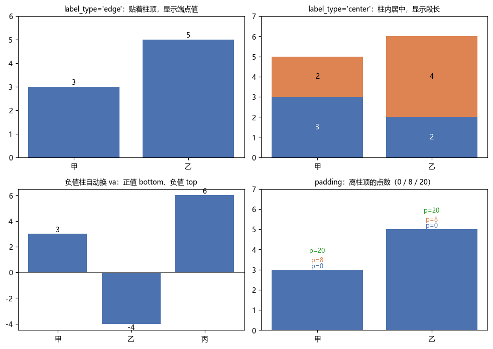
label_type:edge 与 center 显示的根本不是同一个数
这是 bar_label 最容易踩的一处:
import matplotlib.pyplot as plt

fig, ax = plt.subplots()
b1 = ax.bar(['甲', '乙'], [3, 2])
b2 = ax.bar(['甲', '乙'], [2, 4], bottom=[3, 2])

print([t.get_text() for t in ax.bar_label(b2)])
# 输出: ['5', '6']       ← edge:累计的端点高度
print([t.get_text() for t in ax.bar_label(b2, label_type='center')])
# 输出: ['2', '4'] ← center:这一段自身的长度edge 拿的是柱子的上边界坐标,center 拿的是 abs(y0 - y1)(段长)。堆叠柱想标每段的值必须用 center,否则显示的是一层层累加的高度。
center 的锚点坐标看着很怪——两根柱子都报 (0.5, 0.5):
import matplotlib.pyplot as plt

fig, ax = plt.subplots()
b = ax.bar(['甲', '乙'], [3, 5])
fig.canvas.draw()
r = ax.bar_label(b, label_type='center')
print([t.xy for t in r])
# 输出: [(0.5, 0.5), (0.5, 0.5)]因为 center 用的是每根柱子自己的 bbox做变换(源码里是一段按 bar 闭包出来的 xycoords),(0.5, 0.5) 就是「这根柱子的正中间」,跟 axes 坐标无关。
fmt:三种写法,外加可调用对象
import matplotlib.pyplot as plt

fig, ax = plt.subplots()
b = ax.bar(['甲', '乙'], [3, 2])

print([t.get_text() for t in ax.bar_label(b)])
# 输出: ['3', '2']                    ← 默认 fmt='%g'
ax.bar_label(b, fmt='%.1f%%')         # 3.0% / 2.0%
ax.bar_label(b, fmt='{:.2f}')         # 3.00 / 2.00
print([t.get_text() for t in ax.bar_label(b, fmt=lambda v: f'{v / 10:.0%}')])
# 输出: ['30%', '20%']fmt 是字符串时先试 %-style,再试 {}-style;两种都能解释的写法优先按 %-style 处理。所以 '{:.2f}' 和 '%.2f' 都行,'%d 万' 这种带单位后缀的只有 %-style 能做。需要复杂逻辑就传函数(3.7+)。
padding:单位是点,不是数据单位
import matplotlib.pyplot as plt

fig, ax = plt.subplots()
b = ax.bar(['甲', '乙'], [3, 5])

ax.bar_label(b, padding=0)    # 贴住柱顶,字的下缘可能压线
ax.bar_label(b, padding=8)    # 离柱顶 8pt
ax.bar_label(b, padding=20) # 明显上移,适合大字号padding 只改「偏移量」,不改 .xy——.xy 永远是柱子端点。所以想读真实落点得看 get_window_extent(),不是 .xy。
字号调大后 padding=0 会被柱子顶穿,一般跟着 fontsize 一起加:fontsize=9 → padding=3,fontsize=14 → padding=7。
负值柱:va 自动翻转
import matplotlib.pyplot as plt

fig, ax = plt.subplots()
b = ax.bar(['甲', '乙'], [3, -4])
r = ax.bar_label(b, fmt='%.0f')
print([t.get_va() for t in r])
# 输出: ['bottom', 'top']正值柱 va='bottom'(字在柱顶之上),负值柱 va='top'(字在柱底之下)——不需要手动判断。同理 barh 里 ha 也会翻转。
这也是为什么 bar_label 不接受 ha / va:它要按正负自动算。
pie_label():3.11 才有的 API
饼图的 texts / autotexts 手动定位很烦,3.11 加了 pie_label:
w, _ = ax.pie([35, 25, 20, 20])
ax.pie_label(w, ['直销', '渠道', '线上', '其他'], distance=1.15)
# 需要 matplotlib >= 3.11;3.10 会 AttributeError
在 3.10 上它会报:
print(hasattr(plt.matplotlib.axes.Axes, 'pie_label'))
# 输出: False
3.10 及以下的替代方案是 pie(..., autopct='%1.1f%%') 加 wedgeprops,或者拿 autotexts 逐个 set_position。想用新 API 就升级到 3.11+。
返回对象
import matplotlib.pyplot as plt

fig, ax = plt.subplots()
b = ax.bar(['甲', '乙'], [3, 5])
r = ax.bar_label(b, fmt='%.0f')
print(type(r).__name__, len(r), type(r[0]).__name__)
# 输出: list 2 Annotation

print([t.get_text() for t in r])
# 输出: ['3', '5']返回的是 Annotation 列表,和 annotate() 返回的是同一个类——所以 set_text / set_color / set_annotation_clip 全都能用:
import matplotlib.pyplot as plt

fig, ax = plt.subplots()
b = ax.bar(['甲', '乙'], [3, 5])
r = ax.bar_label(b, fmt='%.0f')
r[0].set_color('#c92a2a')
r[1].set_text('5(最高)')
print([t.get_text() for t in r])
# 输出: ['3', '5(最高)']标签被裁掉时统一关掉裁剪:
import matplotlib.pyplot as plt

fig, ax = plt.subplots()
b = ax.bar(['甲', '乙'], [3, 5])
r = ax.bar_label(b, fmt='%.0f')
for t in r:
    t.set_annotation_clip(False)
print([t.get_annotation_clip() for t in r])
# 输出: [False, False]注意事项
- 第一个参数必须是
BarContainer(ax.bar()的返回值)。传ax报AttributeError: 'Axes' object has no attribute 'datavalues',传ax.patches报'ArtistList' object has no attribute 'patches'。 - 显式传
ha/va会抛ValueError: Passing 'ha' to bar_label() is not supported.——对齐是自动按正负号算的。 - 堆叠柱用默认
label_type='edge'显示的是累计高度,不是段长;要段长必须label_type='center'。 label_type='center'的.xy恒为(0.5, 0.5),因为坐标是相对每根柱子自己的 bbox。padding单位是点,不是数据单位;它只改偏移,不改.xy。- 标签默认会被轴范围裁掉,用
ax.set_ylim(0, max*1.15)或ax.margins(y=.1)留白,或逐条set_annotation_clip(False)。 pie_label需要 3.11+;3.10 上hasattr(Axes, 'pie_label')为False。fmt是字符串时 %-style 优先于 {}-style,'%g'与'{:g}'效果相同但前者先命中。
综合示例:柱状 / 堆叠 / 横向三栏
import matplotlib.pyplot as plt
import numpy as np

fig, axes = plt.subplots(1, 3, figsize=(13, 3.6))

# ① 单层柱:端点标注 + 百分比
ax = axes[0]
vals = [35, 25, 20, 20]
b = ax.bar(['直销', '渠道', '线上', '其他'], vals, color='#4C72B0')
ax.bar_label(b, fmt='%d', padding=3)
ax.set_ylim(0, 42)
ax.set_title('label_type=edge', fontsize=9)

# ② 堆叠柱:段内居中,标段长
ax = axes[1]
a = [20, 15, 10]
c = [10, 8, 6]
b1 = ax.bar(['A', 'B', 'C'], a, color='#4C72B0', label='线上')
b2 = ax.bar(['A', 'B', 'C'], c, bottom=a, color='#DD8452', label='线下')
ax.bar_label(b1, label_type='center', fmt='%d', color='white')
ax.bar_label(b2, label_type='center', fmt='%d')
ax.legend(frameon=False, fontsize=8)
ax.set_title("label_type='center'", fontsize=9)

# ③ 横向柱:负值自动翻转 ha
ax = axes[2]
delta = [12, -8, 5]
b = ax.barh(['Q1', 'Q2', 'Q3'], delta,
            color=['#4C72B0' if v > 0 else '#C44E52' for v in delta])
ax.bar_label(b, fmt='%+.0f%%', padding=4, fontsize=9)
ax.axvline(0, color='0.3', lw=.8)
ax.set_title('barh + 负值自动对齐', fontsize=9)

plt.tight_layout()
plt.show()第 ③ 格的关键在于不用写 ha:barh 里正值标签在柱右、负值在柱左,bar_label 按数据正负自己翻。
参考线与阈值:axhline / axvline / axhspan / axvspan / axline
这一组全是「在图上加一条不受数据影响的辅助线/带」。它们的共同点是第一个参数不是 x, y 而是单个阈值,而且短路方向的范围默认用轴比例(0~1)而不是数据坐标。
Axes.axhline(y=0, xmin=0, xmax=1, **kwargs)        # 水平线,贯穿左右
Axes.axvline(x=0, ymin=0, ymax=1, **kwargs)        # 垂直线,贯穿上下
Axes.axhspan(ymin, ymax, xmin=0, xmax=1, **kwargs) # 水平色带
Axes.axvspan(xmin, xmax, ymin=0, ymax=1, **kwargs) # 垂直色带
Axes.axline(xy1, xy2=None, *, slope=None, **kwargs)  # 3.4+:过点或给斜率
Axes.hlines(y, xmin, xmax, **kwargs)   # 数据坐标,可一次画多条
Axes.vlines(x, ymin, ymax, **kwargs) # 数据坐标,可一次画多条| 函数 | 位置参数 | 跨度参数(轴比例) | 返回 |
|---|---|---|---|
axhline |
y 一个值 |
xmin / xmax |
Line2D |
axvline |
x 一个值 |
ymin / ymax |
Line2D |
axhspan |
ymin / ymax |
xmin / xmax |
Rectangle |
axvspan |
xmin / xmax |
ymin / ymax |
Rectangle |
axline |
xy1 + (xy2 或 slope) |
无限延伸 | AxLine |
hlines |
y 列表 |
xmin / xmax(数据) |
LineCollection |
vlines |
x 列表 |
ymin / ymax(数据) |
LineCollection |
最小示例
import matplotlib.pyplot as plt
import numpy as np

rng = np.random.default_rng(0)
x = rng.normal(size=300)
fig, ax = plt.subplots()
ax.hist(x, bins=30, color='#4C72B0', alpha=.75)

m, s = x.mean(), x.std()
ax.axvline(m, color='crimson', lw=2, ls='--', label=f'均值 {m:.2f}')
ax.axvspan(m - s, m + s, color='tab:green', alpha=.15, label='±1σ')
ax.axhline(20, color='gray', ls='-.', lw=1)
ax.legend()
plt.show()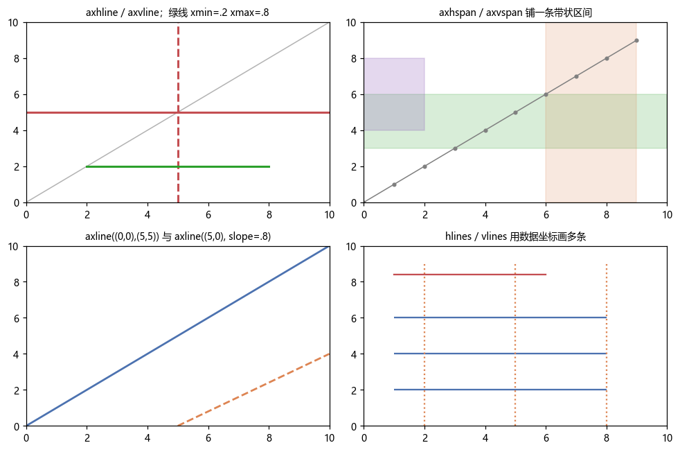
xmin / xmax 是轴比例,不是数据坐标
这是最容易搞混的一点。axhline(y=5, xmin=0.2, xmax=0.8) 画的线不是从 x=0.2 到 x=0.8,而是从「轴宽的 20%」到「80%」:
import matplotlib.pyplot as plt

fig, ax = plt.subplots()
ax.set_xlim(0, 10)
ln = ax.axhline(5, xmin=0.2, xmax=0.8)
print(ln.get_xdata())
# 输出: [0.2, 0.8] ← 存的就是比例值要按数据坐标指定起点终点,用 hlines / vlines:
import matplotlib.pyplot as plt

fig, ax = plt.subplots()
hl = ax.hlines([2, 4], xmin=3, xmax=7)
print([(s[0].tolist(), s[1].tolist()) for s in hl.get_segments()])
# 输出: [([3.0, 2.0], [7.0, 2.0]), ([3.0, 4.0], [7.0, 4.0])]
hlines 的 y 可以是列表(一次画多条),返回 LineCollection 而不是 Line2D。要单独改某一条得用 set_color() 传颜色列表,不能下标索引。
axline:过两点或给斜率,二选一
ax.axline((0, 0), (5, 5))        # 过 (0,0) 和 (5,5)
ax.axline((5, 0), slope=0.8)     # 过 (5,0)、斜率 0.8
xy2 和 slope 必须给且只能给一个:
import matplotlib.pyplot as plt

fig, ax = plt.subplots()
try:
    ax.axline((1, 1))
except TypeError as e:
    print(e)
# 输出: Exactly one of 'xy2' and 'slope' must be givenaxline 是无限延伸的(画到轴边界为止),这点和 axhline 一样,但方向任意。要限定区间还是得回到 plot 或 hlines。
色带 axhspan / axvspan:标注「某个区间」
ax.axhspan(3, 6, color='tab:green', alpha=.15)              # 整条水平带
ax.axvspan(6, 9, color='tab:orange', alpha=.15)             # 整条垂直带
ax.axvspan(0, 2, ymin=.4, ymax=.8, color='tab:purple', alpha=.25)  # 只占下半段
axhspan 的两个位置参数是数据坐标的 y 范围,跨度参数 xmin/xmax 仍是轴比例;axvspan 反过来。返回的是 Rectangle patch,所以 hatch / lw / set_zorder 都能用。
色带上的 alpha 基本必设——默认不透明会盖住底下的数据。
样式:全部沿用 plot 的关键字
ax.axvline(3, color='#C44E52', lw=2, ls='--', alpha=.8, zorder=1, label='阈值')color / lw / ls / alpha / zorder / label 全透传给 Line2D。label 给了才会进图例——这是「参考线为什么不显示在图例里」的常见原因。
返回对象
import matplotlib.pyplot as plt

fig, ax = plt.subplots()
ln = ax.axvline(3, color='crimson', lw=2, ls='--')
print(type(ln).__name__)
# 输出: Line2D

sp = ax.axvspan(1, 2, alpha=.2)
print(type(sp).__name__)
# 输出: Rectangleaxhline / axvline 返回 Line2D,所以 set_ydata / set_xdata 能改位置——但 axhline 有个专门的方法更省事:
import matplotlib.pyplot as plt

fig, ax = plt.subplots()
ln = ax.axvline(3)
ln.set_xdata([7, 7])
print(ln.get_xdata())
# 输出: [7, 7]注意 axhline / axvline 的 xdata / ydata 存的是跨度比例(两端各一个值),位置在另一个轴的数据坐标上。所以改 axvline 的位置要调 set_xdata,改它的上下跨度要调 set_ydata。
axline 返回的 AxLine 虽然是 Line2D 的子类,但它的位置每次重绘都从 _point1 / _point2 重算,所以 set_xdata 存在却不起作用:
import matplotlib.pyplot as plt

fig, ax = plt.subplots()
al = ax.axline((1, 1), slope=2)
print(type(al).__name__, hasattr(al, 'set_xdata'))
# 输出: AxLine True

al.set_xdata([5, 9])
print(al.get_xdata())
# 输出: [5, 9] ← 值改了,但直线位置不会跟着动想换位置只能重建 axline(),或者用 plot 画一条普通线。
注意事项
axhline/axvline/axhspan/axvspan的跨度参数是轴比例 0~1,不是数据坐标。按数据坐标画要用hlines/vlines。hlines/vlines返回LineCollection,一次可画多条;axhline一次只能画一条。axline的xy2与slope必须二选一,都给或都不给都是TypeError。axline无限延伸,不能限定区间;要区间用plot。- 色带默认不透明,必须自己加
alpha,否则把数据全盖住。 - 参考线不给
label就不进图例,ax.legend()里找不到它们是正常的。 axhline的zorder默认2,和plot的线一样;想让它压在数据后面写zorder=0或1。- 阈值线随图例变化不会自动更新文字,
label=f'均值 {m:.2f}'只在建线那一刻取值。
综合示例:分布图三件套 / 阈值分区 / 区间底纹
import matplotlib.pyplot as plt
import numpy as np

fig, axes = plt.subplots(1, 3, figsize=(13, 3.8))
rng = np.random.default_rng(7)

# ① 直方图 + 均值线 + ±1σ 色带
ax = axes[0]
x = rng.normal(0, 1, 500)
ax.hist(x, bins=30, color='#4C72B0', alpha=.75)
m, s = x.mean(), x.std()
ax.axvline(m, color='crimson', lw=2, ls='--', label=f'μ={m:.2f}')
ax.axvspan(m - s, m + s, color='tab:green', alpha=.15, label='±1σ')
ax.axvline(m + 2 * s, color='royalblue', lw=1.5, ls=':', label='+2σ')
ax.legend(fontsize=8, frameon=False)
ax.set_title('均值与置信带', fontsize=9)

# ② 阈值分区:用色带铺出「合格 / 预警 / 超标」三段
ax = axes[1]
y = np.cumsum(rng.normal(0, .6, 40))
ax.plot(y, color='#4C72B0', lw=1.6, marker='o', ms=3)
ax.axhspan(0, 3, color='#2ca02c', alpha=.10)
ax.axhspan(3, 5, color='#f08c00', alpha=.10)
ax.axhspan(5, 9, color='#c92a2a', alpha=.10)
for v, t in [(3, '预警线 3'), (5, '超标线 5')]:
    ax.axhline(v, color='0.35', lw=1, ls='--')
    ax.text(.02, v + .12, t, fontsize=8, transform=ax.get_yaxis_transform(), color='0.3')
ax.set_ylim(0, 9)
ax.set_title('阈值分区(axhspan)', fontsize=9)

# ③ 用 hlines 按数据坐标画多条区间参照
ax = axes[2]
vals = [4.2, 6.8, 5.5]
ax.barh(['A', 'B', 'C'], vals, color='#4C72B0', height=.45)
ax.hlines([0, 1, 2], xmin=2, xmax=7, color='0.4', lw=1.2, ls=':')
ax.vlines([2, 7], ymin=-.5, ymax=2.5, color='#C44E52', lw=1.2)
ax.set_xlim(0, 9)
ax.set_title('hlines / vlines:数据坐标 + 多条', fontsize=9)

plt.tight_layout()
plt.show()第 ② 格的 ax.text(..., transform=ax.get_yaxis_transform()) 是配套技巧:x 用轴比例、y 用数据坐标,让标签永远贴在左边框上,不受数据范围影响。